Activation Functions I: Basic AF

Deep learning is actually not a difficult or complicated algorithm. In the whole process of deep learning framework design, the choice of activation function is one of the most critical and technical parts. In this post, we would like to review some commonly used activation functions and give a guideline on how to choose activation functions in different scenarios.
First, we introduce some basic activation functions.
- Step Function
Basically, the activation function should answer the question of whether or not the neuron should take place. A step function can achieve this goal by determining a reliable threshold value \(T\). Then the function can be written as:
\[f(x) = \{0, for x \leq T; 1, for x>T \} \]

The effect of a step function as an activation function is heavily dependent on the threshold. In addition, it is not flexible and hence has numerous challenges during training for the network models.
- Linear Activation Function
Step functions have zero gradients, thus it can not reflect the gradual change of the input. Considering this defection, we would like to give a try the linear functions, which can be expressed as
\[ f(x) = ax, where a \in R\]
Linear functions have a constant derivative function, which makes the descent a constant too. Furthermore, the composite function of linear functions is still a linear function, which makes deep learning with multiple layers meaningless.
- "S"-shaped Activation Functions
These types of activation functions are the most commonly used activation functions in the early machine learning and deep learning world.
3.1. Sigmoid Function
The sigmoid function is a nonlinear function, which makes it a powerful competitor when we need to stack multiple layers of neurons. The equation below demonstrates a simple sigmoid function:
\[ \sigma(x) = \dfrac{1}{1+e^{-x}}\]
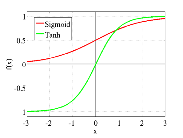
The graph of this function is as beautiful as its expression.
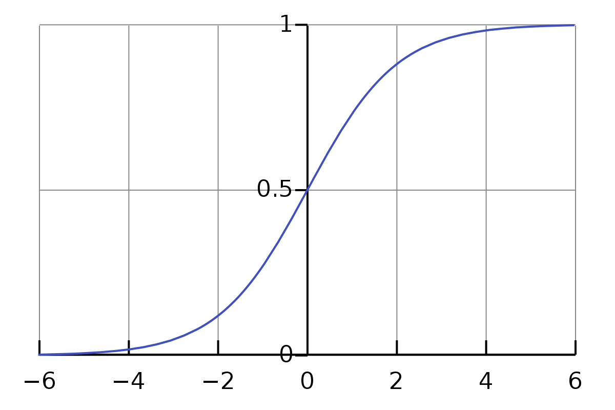
The sigmoid function varies widely when the input value is between -2 and 2, which makes it a great classifier by making clear prediction distinctions.
Moreover, this function has a bounded range of \( (0, 1) \). Therefore, it is easy to prevent blowing up during the activations, and the output value can be regarded as a probability in classification problems.
Despite all advantages mentioned above, the sigmoid function still has its disadvantages. The gradient of the sigmoid function vanishes when input gradually moves away from the origin. In this case, the network can either learn drastically slowly or refuse to learn further. Another issue is that the sigmoid function always produces a non-zero value. That will make the entire training procedure takes more steps to converge than it might need with a more advanced activation.
3.2. Hyperbolic Tangent Activation Function
In order to overcome the disadvantages of the non-zero centrality of the sigmoid function, the hyperbolic function, which is also known as the tanh function, is introduced to the deep learning world. The figure below shows a comparison between the sigmoid and the tanh function.
The form of the tanh function is
\[ f(x) = tanh(x) = \dfrac{e^{x} - {e}^{-x}} {e^{x}+ {e}^{-x}}\]
The tanh function is sigmoidal, however, its values range between -1 and 1, which makes negative inputs of the hyperbolic functions will be mapped to a negative output. Therefore, the network is not stuck due to the above features during training.
Another advantage of tanh is that the derivatives of the tanh are significantly larger than that of the sigmoid near zero. As a consequence, tanh is more helpful when you need to find the local or global minimum quickly.
Despite all the pros, the tanh, just like the sigmoid also struggles with the vanishing gradient problem. Before the savior comes on the scene, we believe that it is worth mentioning a few attempts to upgrade "s"-shaped functions.
3.3. Softsign Activation Function
Softsign, which is smoother than tanh, is one of the most important "s"-shape activation functions. We can get some intuition about the properties of this function from its equation below.
\[f(x) = \dfrac{x}{(1+|x|)}\]
If we plot the tanh and the softsign together, we will find their common points and difference.
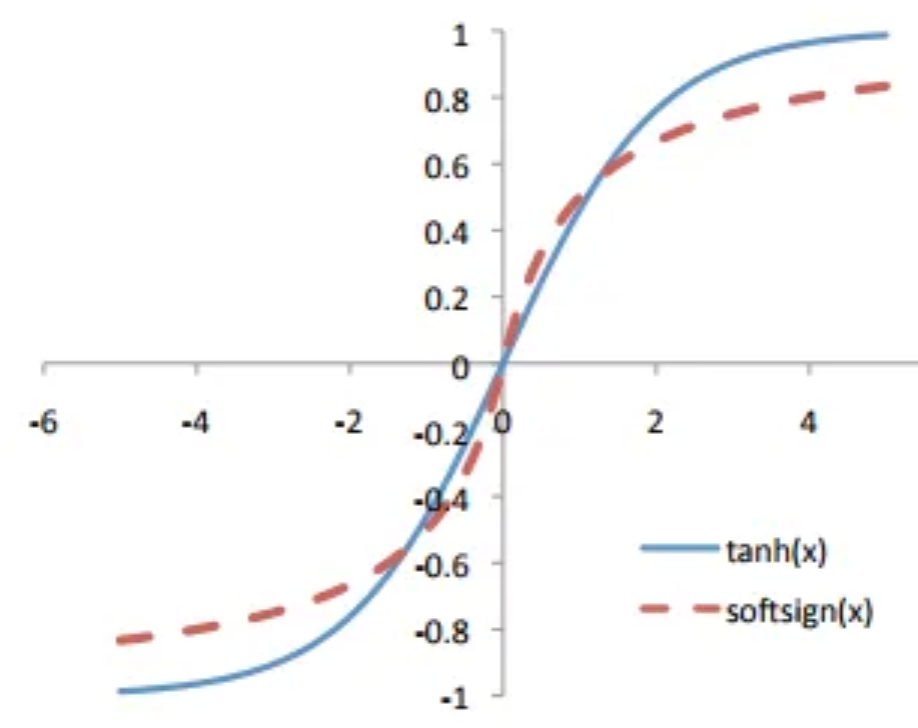
Since Softsign grows polynomially rather than exponentially. This gentler non-linearity results in better and faster learning due to a lack of struggle with vanishing gradients. However, it is more expensive to compute Softsign because it has more complicated derivatives.
Vanishing Gradient Problem
Almost all "s"-shape activation functions suffer from vanishing gradient. We take the sigmoid function and MNIST dataset for example to show how learning speed gradually slow down due to the vanishig gradient problem.
| Number of hidden layers | Accuracy for Sigmoid |
|---|---|
| 1 hidden layer | 96.81% |
| 2 hidden layer | 97.18% |
| 3 hidden layer | 97.29% |
| 4 hidden layer | 97.10% |
You can see that we achieve pretty good accuracy in the single-layer model. Then the accuracy grows a little bit for 2 and 3 layers, but for the four hidden layers, the accuracy rate drops down back and has a worse performance even than 2 layers model.
This degeneration roots from the vanishing gradient of the sigmoid function, which can be avoided by using functions with static or wider-range derivatives.
- Rectified Linear Unit Activation Function
In general, this type of activation function is responsible for transforming the weighted input that is summed up from the node to the strict output or proportional sum. These functions are piecewise linear functions that usually output the positive input directly; otherwise, its output is zero.
4.1. Rectified Linear Unit (ReLU)
The equation below demonstrates a basic ReLU function:
\[f(x) = x ^ {+} = max (0, x)\]
I believe the function above is not a "new" function for most of the readers. It is also called a ramp function, which is used in electrical engineering as half-wave rectification, in statistics as the Tobit model, and in financial engineering as call option payoff.
It has been proven to be more efficient than the sigmoid or the hyperbolic tangent functions. Moreover, the cost of computing the derivative and gradient is fairly low. The results from some research show that ReLU and its minor variants are hard to beat in solving classification problems.
Nothing is perfect, ReLU has its own shortcoming known as "dying ReLU". Although the theoretical explanation of "dying ReLU" might be unnecessary to put here, you can predict that ReLU would have a strange behavior when the inputs are approaching the kink point. When the inputs fall to the left of the origin, no matter how much it changes, ReLU will not give any reflection at all.
4.2. Leaky Rectified Linear Unit
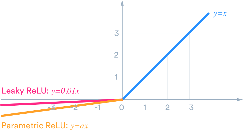
To avoid "dying ReLU", we need to reduce the possibility of returning 0 value as output. That could be achieved by making a small change to the function. Leaky ReLU and its more general version, parametric ReLU can be written as:
\[f(x) = \{\alpha * x, for x \leq 0; x, for x>0 \}\]
where \(\alpha\) equals \(0.01\) in the leaky ReLU and has no specific restriction for parametric ReLU.
- Softplus Activation Function
Another alternative to basic ReLU is Softplus. It is also described as a better alternative to sigmoid or tanh. Softplus also has two versions. One is the basic Softplus, which can be written as:
\[f(x) = ln(1 + e^{x})\]
The other one is the parametric Softplus:
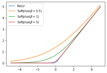
\[ f(x) = \dfrac{1}{\beta} * log(1 + exp(\beta * x) ) \]
where \(\beta\) is a tunable positive parameter. The properties of the Softplus function are mainly dependent on the value of \(\beta\). As \(\beta\) approaches zero, the Softplus function behaves like a linear activation function. On the other hand, when \(\beta \rightarrow \infty\), it performs more like a basic ReLU.
One of the biggest pros for Softplus is its smooth derivative used in backpropagation. Moreover, the local minima of greater or equal quality, are attained by the network trained with the rectifier activation function despite the hard threshold at zero.
- Swish Activation Function
Another powerful alternative to ReLU is invented by the Google brain team, the swish activation function. Swish activation function is represented by the equation below:
\[f(x) = x * \sigma(x) = \dfrac{x}{1+e^{-x}}\]
Swish also has its parametric modification, which has the form below:
\[f(x) = \beta x * \sigma(\beta x) = \dfrac{\beta x}{1 + e^{-\beta * x}}\]
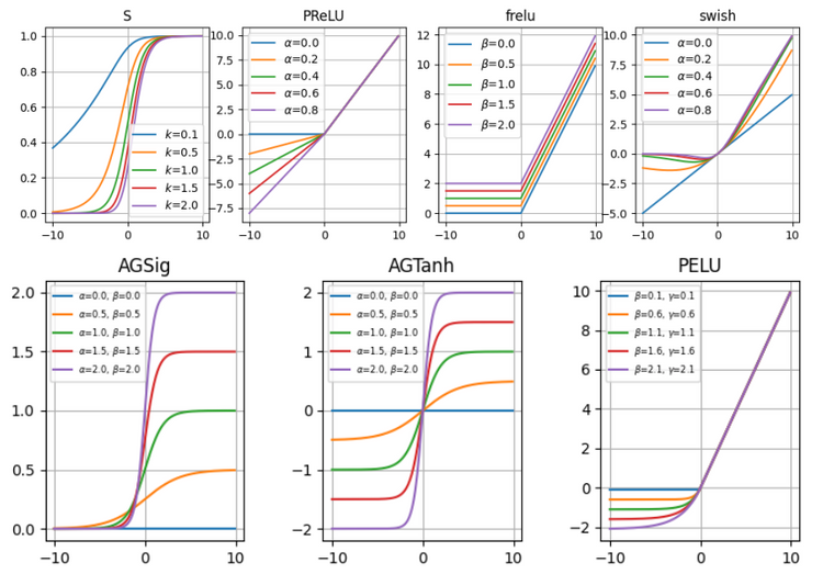
The figure below shows what different graphs the parametric Swish functions can produce via using different values of beta.
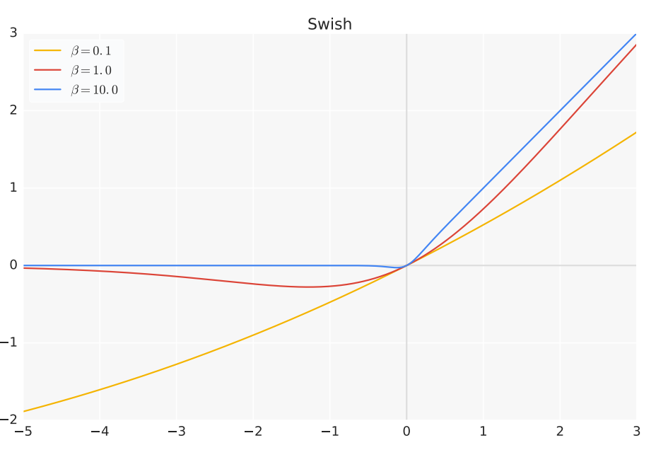
A linear function will be attained if \(\beta\) is moved closer to zero; meanwhile, the function will look like ReLU if \(\beta\) gets closer to one.
The Swish function is easily derivable. Moreover, experiments prove that Swish performs better than the ReLU -- so far the most efficient activation function of deep learning.
Conclusions
We investigate many different activation functions in this post. Since each function has its own pros and cons, there is no dominant activation function that can beat other activation functions under any circumstances. We list all activation functions mentioned in this post in the table below and give recommendations on when to use which one.
| Activation Function | Main Comment | Use Case |
|---|---|---|
| Step | Does not work with the backpropagation algorithm | Rather never |
| Sigmoid | Prone to the vanishing gradient function and zigzagging during training due to not being zero centered | Can be used as logic gates |
| Tanh | Also prone to vanishing gradient | RNN |
| Softsign | Similar to tanh | No special use case |
| ReLU | The most popular function for hidden layers. Although, under rare circumstances, is prone to the "Dying ReLU" problem. | First to go choice |
| Leaky ReLU | Comes with all pros of ReLU, but due to not-zero output will never "die" | Use only if you expect the "Dying ReLU" problem |
| Maxout | Far more advanced activation function than ReLU, immune to "Dying ReLU", but much more expensive in case of computation | Use as a last resort |
| Softplus | Similar to ReLU, but a bit smoother near 0. Comes with comparable benefits as ReLU, but has a more complex formula, therefore producing a slower network. | Rather never |
| Swish | Similar as leaky ReLU, not outperform ReLU. Might be more useful in networks with dozens of layers. | Worth to give a try in very deep networks |
| SoftMax | A generalization of the logistic function to multiple dimensions. | For the output layer in classification networks |
| OpenMax | Enable to estimate the probability of an input being from an unknown class, allow rejection of "fooling" and unrelated samples presented to the system. | For the output layer in classification with open classes possibility. |
Reference:
- Review and Comparison of Commonly Used Activation Functions for DeeP Neural Networks, Tomasz Szanda.
- Wikipedia.