
Assessing Reliability: A Review of Failure Rates in Large-Scale IT System

1. Introduction
As the complexity of large-scale IT infrastructures increases, with clusters encompassing millions of components, the challenge of managing component failures has evolved from a mere technical hurdle to a critical business imperative. In such expansive systems, ensuring high reliability is not only technically challenging but also carries substantial financial implications, particularly in terms of disaster prevention and recovery costs.
This challenge is acutely felt across various sectors, such as high-performance computing and internet service provision, where hardware failures can cause significant operational disruptions, degrade end-user experiences, and tarnish business reputations.
The ability to understand, predict, and effectively manage these failures is therefore not just a technical necessity but a strategic asset. It enhances operational resilience, drives smarter engineering practices, and leads to more cost-effective hardware solutions.
In this document, we delve into the foundational concepts of component failure rates, drawing upon extensive research from industry leaders and academia. We aim to present a thorough analysis of the challenges and innovative solutions in maintaining hardware reliability within large-scale IT systems. Furthermore, this document sets the stage for our own future research initiatives at ApexCDS. We intend to develop predictive models for failure forecasting, significantly contributing to the optimization of our supply chain and overall operational efficiency through data-driven strategies.
2. Understanding Failure Rates: Key Concepts and Practical Implication
When managing large-scale IT systems, it’s crucial to understand the concepts that describe and quantify system failures. Here’s a breakdown of the most important terms:
Reliability: This is like asking, “What are the odds this component will work without a hitch for a certain time under normal conditions?” For example, if a hard drive has high reliability, it’s likely to function well for several years.
Mean time between failures (MTBF) is the predicted elapsed time between inherent failures of a mechanical or electronic system during normal system operation. Imagine a group of servers in a data center.
MTBF tells us, on average, how long it takes for one of these servers to encounter a problem during normal operation. It’s calculated by averaging the time intervals between failures. For instance, if three servers fail after 100, 200, and 300 hours respectively, the MTBF would be (100+200+300)/3 = 200 hours.
MTBF can be calculated as the arithmetic mean (average) time between failures of a system.
$$\text{MTBF} = \frac{\sum (\text{start of downtime} - \text{start of uptime})}{\text{number of failures}}$$
Mean time to failure (MTTF): This is used for items that aren’t repaired once they fail, like a disposable battery. MTTF is the average time until such an item fails. So, if a type of battery typically lasts around 500 hours, that would be its MTTF.
Failure rate: This is a bit like asking, “Given that this device was working fine at the beginning of the year, what’s the chance it will fail by the end of the year?” This rate changes over the product’s lifetime.
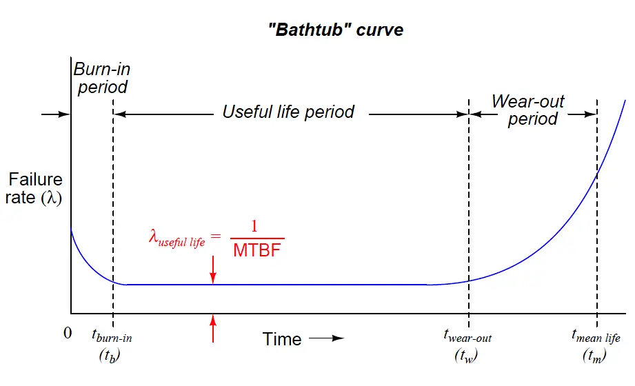
These concepts help us understand a product’s lifecycle, often illustrated as a “bathtub curve” with three phases:
-
Burn-in: Early life, where defects might cause some components to fail. It’s like a new car having issues in the first few months.
-
Useful Life: The period when the component is most reliable and failures are less frequent and random.
-
Wear-out: When components get old and wear out, failures become more common again.
For example, a new HDD might have some initial failures (burn-in), then work reliably for years (useful life), and finally start to fail as it gets old (wear-out).
Let reliability be represented by $R(t)$and failure rate by $F(t)$. Using Weibull distribution, they can be quantified as follows:
$$R(t)=e^{-\lambda t^{\beta}}\text{ and }F(t)=\lambda\beta t^{\beta-1}.$$
Remember, reliability is the probability that a part will function at least a specified time. Failure rate describes the frequency with which failures can be expected to occur. The values of the parameters in the above expression are not always the same at different periods of a component's life cycle.
The life cycle of a part can be divided into three distinct periods: burn-in, useful life, and wear-out. These three periods are characterized mathematically by a decreasing failure rate, a constant failure rate, and an increasing failure rate, which can be illustrated as a "bathtub curve" below.
The listed formulae can model all three of these phases by picking appropriate value of the parameters.
-
- When $\beta<1$, $F(t)$ becomes a decreasing function, which can be used to describe the 'burn-in' stage.
-
- When $\beta=1$, $F(t)$ is a constant number, which corresponds to the 'useful life' stage.
-
- When $\beta>1$, $F(t)$ becomes an increasing function, which is exactly the case as the 'wear-out' stage.
Given good design, debugging, and thorough testing of product, the burn-in period of a part's life should be passed by the time the parts are shipped. Therefore, we can assume that most failures occur during the useful life phase, and result, not from a systematic defect, but rather from random causes which have a constant failure rate. The constant failure rate presumption results in $\beta=1$. Thus
$$F(t)=\lambda$$
The concept of a constant failure rate says that failures can be expected to occur at equal intervals of time. Under these conditions, the mean time to the first failure, the mean time between failures, and the average life time are all equal. Thus, the failure rate in failures per $\text{device}\cdot\text{hour}$, is simply the reciprocal of the number of $\text{device}\cdot\text{hours}$ per failure. That is
$$F(t)=\lambda\approx\frac{1}{\text{MTTF}}$$
during constant failure rate conditions.
While conducting failure rate analysis or research in the field, it's often challenging to pinpoint the exact time of failure. Therefore, we sometimes resort to measurable metrics as proxies for failure rate, such as replacement rate, repair request rate, or error report rate, among others. The choice of proxy depends on the specific IT systems and the components under investigation. In the review that follows, we will clearly specify each proxy used to avoid any confusion.
3. Overview of Existing IT System Failure Studies
Carnegie Mellon University (2007)
- Article Title: What does an MTTF of 1,000,000 hours mean to you?
- Component under Investigation: HDD
- Scale: More than 100,000 drives
- Data sources:
- Data sets HPC1, HPC2, HPC3 were collected in three large cluster systems at three different organizations using supercomputers. Data set HPC4 was collected on dozens of independently managed HPC sites, including supercomputing sites as well as commercial HPC sites.
- Data sets COM1, COM2, and COM3 were collected in at least three different cluster systems at a large internet service provider with many distributed and separately managed sites.
- In all cases, their data reports on only a portion of the computing systems run by each organization, as decided and selected by our sources.
- AFR proxies: Annual replacement rate (ARR)
- Key Findings:
- Observation 1: Variance between datasheet MTTF and disk replacement rates in the field was larger than we expected. The weighted average ARR was 3.4 times larger than 0.88%, corresponding to a datasheet MTTF of 1,000,000 hours.
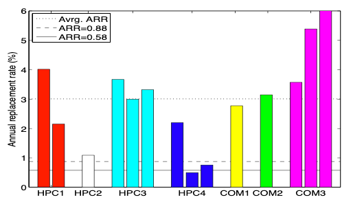
Figure: Comparison of datasheet AFRs (solid and dashed line in the graph) and ARRs observed in the field.
- Observation 2: For older systems (5-8 years of age), data sheet MTTFs underestimated replacement rates by as much as a factor of 30.
- Observation 3: Even during the first few years of a system’s lifetime (< 3 years), when wear-out is not ex- pected to be a significant factor, the difference between datasheet MTTF and observed time to disk replacement was as large as a factor of 6.
- Observation 4: In our data sets, the replacement rates of SATA disks are not worse than the replacement rates of SCSI or FC disks. This may indicate that disk-independent factors, such as operating conditions, usage and environmental factors, affect replacement rates more than component specific factors. However, the only evidence we have of a bad batch of disks was found in a collection of SATA disks experiencing high media error rates. We have too little data on bad batches to estimate the relative frequency of bad batches by type of disk, although there is plenty of anecdotal evidence that bad batches are not unique to SATA disks.
- Observation 5: Contrary to common and proposed models, hard drive replacement rates do not enter steady state after the first year of operation. Instead replacement rates seem to steadily increase over time.
- Observation 6: Early onset of wear-out seems to have a much stronger impact on lifecycle replacement rates than infant mortality, as experienced by end customers, even when considering only the first three or five years of a system’s lifetime. We therefore recommend that wear-out be incorporated into new standards for disk drive reliability. The new standard suggested by IDEMA does not take wear-out into account.
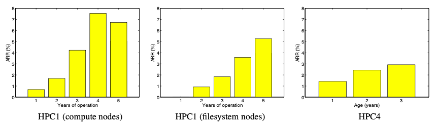
Figure: ARR for the first five years of system HPC1’s lifetime, for the compute nodes (left) and the file system nodes (middle). ARR for the first type of drives in HPC4 as a function of drive age in years (right).
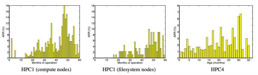
Figure: ARR per month over the first five years of system HPC1’s lifetime, for the compute nodes (left) and the file system nodes (middle). ARR for the first type of drives in HPC4 as a function of drive age in months (right).
- Observation 7: Disk replacement counts exhibit significant levels of autocorrelation.
- Observation 8: Disk replacement counts exhibit long-range dependence.
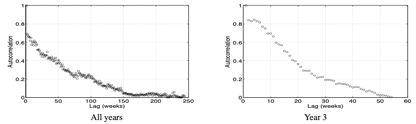
Figure: Autocorrelation function for the number of disk replacements per week computed across the entire lifetime of the HPC1 system (left) and computed across only one year of HPC1’s operation (right).
- Observation 9: The hypothesis that time between disk replacements follows an exponential distribution can be rejected with high confidence.
- Observation 10: The time between disk replacements has a higher variability than that of an exponential distribution.
- Observation 11: The distribution of time between disk replacements exhibits decreasing hazard rates, that is, the expected remaining time until the next disk was replaced grows with the time it has been since the last disk replacement.
Google (2007)
- Article Title: Failure Trend in a Large Disk Drive Population
- Component under Investigation: HDD
- Scale: More than 100,000 drives
- Data sources:
- "We present data collected from detailed observations of a large disk drive population in a production Internet services deployment. "
- AFR proxies: Annual replacement rate (ARR)
- Key Findings:
- “Contrary to previously reported results, we found very little correlation between failure rates and either elevated temperature or activity levels. ”
Utilization AFR
AFR for average drive temperature
- Some SMART parameters (scan errors, reallocation counts, offline reallocation counts, and probational counts) have a large impact on failure probability. (SMART: A driver's self monitoring facility.)
AFR for scan errors
AFR for reallocation counts
- Given the lack of occurrence of predictive SMART signals on a large fraction of failed drives, it is unlikely that an accurate predictive failure model can be built based on these signals alone.
Microsoft (2010)
- Article Title: Characterizing Cloud Computing Hardware Reliability
- Component under Investigation: Server
- Scale: Over 100,000
- Data sources: Ideally we would have access to detailed logs corresponding to every hardware repair incident during the lifetime of the servers. We would also know when the servers were comissioned and de- comissioned. However, without the proven need for such detailed logging no such database exists. Thus, in the absence we resort to combining multiple data sources to glean as much information as we can.
- The first piece of data is the inventory of machines.
- The next piece of information that is critical is the hardware replacements that take place.
- AFR proxies: ARR
- Key Findings:
- "We find that (similar to others) hard disks are the number one replaced components, not just because it is the most dominant component but also because it is one of the least reliable. "
- We find that 8% of all servers can expect to see at least 1 hardware incident in a given year and that this number is higher for machines with lots of hard disks.
- We can approximate the IT cost due to hardware repair for a mega datacenter (> 100,000 servers) to be over a million dollars.
- Furthermore, upon seeing a failure, the chances of seeing another failure on the same server is high.
- We find that the distribution of successive failure on a machine fits an inverse curve. Our initial hypothesis is that upon seeing a failure the machine makes a transition from a benign state to a new state where there is a rich structure in failure patterns.
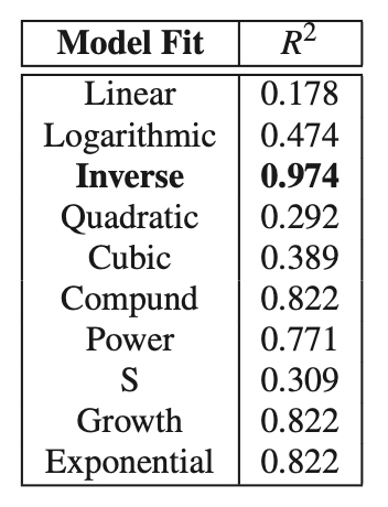
Table: $R^2$ values for various statistical curves fit against days between successive failures on the same machine.
- We also find that, location of the datacenter and the manufacturer are the strongest indicators of failures, as opposed to age, configuration etc.
Facebook (2015)
- Article Title: A Large-Scale Study of Flash Memory Failures in the Field
- Component under Investigation: SSD
- Scale: Many millions of SSDs
- Data sources:
- The flash devices in our fleet contain registers that keep track of statistics related to SSD operation (e.g., number of bytes read, number of bytes written, number of uncorrectable errors). These registers are similar to, but distinct from, the standardized SMART data stored by some SSDs to monitor their reliability characteristics. The values in these registers can be queried by the host machine. We use a collector script to retrieve the raw values from the SSD and parse them into a form that can be curated in a Hive table. This process is done in real time every hour.
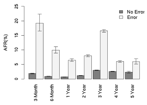
- AFR proxies: "We refer to the occurrence of such uncorrectable errors in an SSD as an SSD failure. "
- Key Findings:
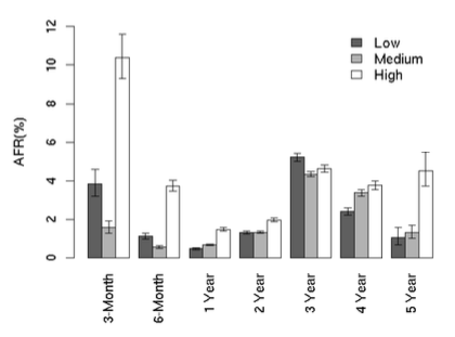
- SSD failures are relatively common events with between 4.2% and 34.1% of the SSDs in the platforms we examine reporting uncorrectable errors.
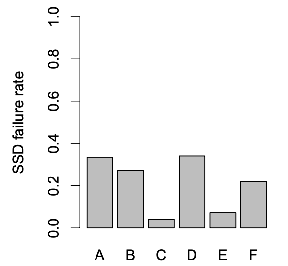
SSD Failure Rate
- SSD failure rates do not increase monotonically with flash chip wear; instead they go through several distinct periods corresponding to how failures emerge and are subsequently detected.
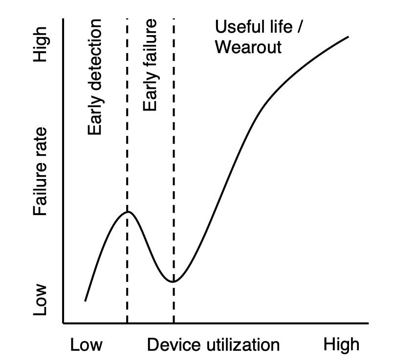
Figure: SSDs fail at different rates during several distinct periods throughout their lifetime (which we measure by usage): early detection, early failure, useful life, and wearout.
- The effects of read disturbance errors are not prevalent in the field.
- Sparse logical data layout across an SSD’s physical address space (e.g., non-contiguous data), as measured by the amount of metadata required to track logical address translations stored in an SSD-internal DRAM buffer, can greatly affect SSD failure rate.
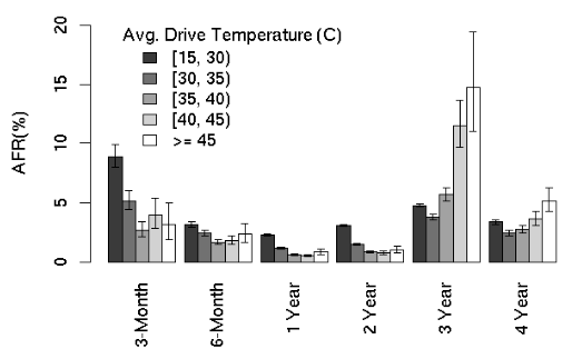
- Higher temperatures lead to higher failure rates, but techniques that throttle SSD operation appear to greatly reduce the negative reliability impact of higher temperatures.
- Data written by the operating system to flash-based SSDs does not always accurately indicate the amount of wear induced on flash cells due to optimizations in the SSD controller and buffering employed in the system software.
- We also find that the distribution of number of errors among SSDs in a platform is similar to that of a Weibull distribution with a shape parameter of 0.3 and scale parameter of $5\times 10^{3}$. The solid black line on the figure below plots this distribution.
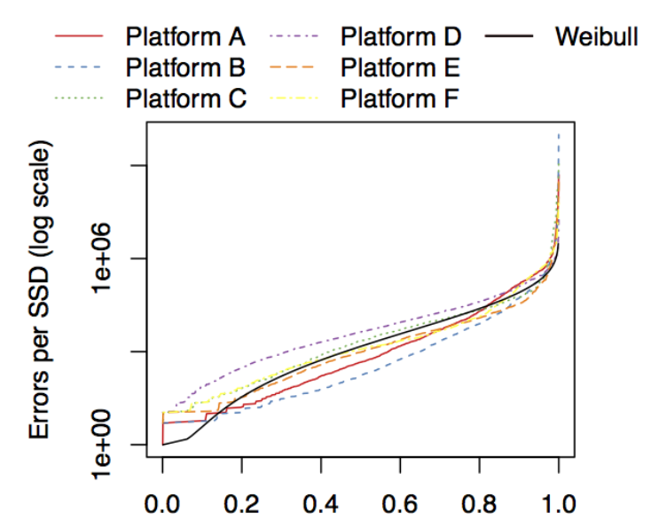
Figure: The distribution of uncorrectable error count across SSDs
Google (2016)
- Article Title: Flash Reliability in Production: The Expected and the Unexpected
- Component under Investigation: SSD
- Scale: Many millions of drive days
- Data sources:
- The data was collected over a 6-year period and contains for each drive aggregated monitoring data for each day the drive was in the field.
- Besides daily counts for a variety of different types of errors, the data also includes daily workload statistics, including the number of read, write, and erase operations, and the number of bad blocks developed during that day. The number of read, write, and erase operations includes user-issued operations, as well as internal operations due to garbage collection.
- Another log records when a chip was declared failed and when a drive was being swapped to be repaired.
- AFR proxies: The field characteristics of different types of hardware failure, including block failures, chip failures and the rates of repair and replacement of drives.
- Key Findings:
- We find that the flash drives in our study experience significantly lower replacement rates (within their rated lifetime) than hard disk drives. On the downside, they experience significantly higher rates of uncor-rectable errors than hard disk drives.
- Between 20–63% of drives experience at least one uncorrectable error during their first four years in the field, making uncorrectable errors the most common non-transparent error in these drives. Between 2–6 out of 1,000 drive days are affected by them.
- The majority of drive days experience at least one correctable error. However, other types of transparent errors, i.e. errors which the drive can mask from the user, are rare compared to non-transparent errors.
- We find that RBER (raw bit error rate), the standard metric for drive reliability, is not a good predictor of those failure modes that are the major concern in practice. In particular, higher RBER does not translate to a higher incidence of uncorrectable errors.
- Both RBER and the number of uncorrectable errors grow with PE cycles, however the rate of growth is slower than commonly expected, following a linear rather than exponential rate, and there are no sudden spikes once a drive exceeds the vendor’s PE cycle limit, within the PE cycle ranges we observe in the field.
- While wear-out from usage is often the focus of attention, we note that independently of usage the age of a drive, i.e. the time spent in the field, affects reliability.
- SLC drives, which are targeted at the enterprise market and considered to be higher end, are not more reliable than the lower end MLC drives.
- We observe that chips with smaller feature sizes tend to experience higher RBER, but are not necessarily the ones with the highest incidence of non-transparent errors, such as uncorrectable errors.
- While flash drives offer lower field replacement rates than hard disk drives, they have a significantly higher rate of problems that can impact the user, such as uncorrectable errors.
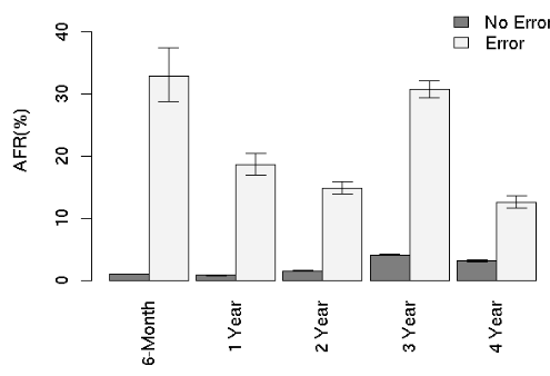
- Previous errors of various types are predictive of later uncorrectable errors. (In fact, we have work in progress showing that standard machine learning techniques can predict uncorrectable errors based on age and prior errors with an interesting accuracy.)
- Bad blocks and bad chips occur at a significant rate: depending on the model, 30-80% of drives develop at least one bad block and 2-7% develop at least one bad chip during the first four years in the field. The latter emphasizes the importance of mechanisms for mapping out bad chips, as otherwise drives with a bad chips will require repairs or be returned to the vendor.
- Drives tend to either have less than a handful of bad blocks, or a large number of them, suggesting that impending chip failure could be predicted based on prior number of bad blocks (and maybe other factors). Also, a drive with a large number of factory bad blocks has a higher chance of developing more bad blocks in the field, as well as certain types of errors.
Microsoft (2016)
- Article Title: SSD Failures in Datacenters: What? When? and Why?
- Component under Investigation: SSD
- Scale: Half a million SSDs
- Data sources: Runtime collects data for monitoring system health and performance issues through various sources in the datacenter.
- SMART monitoring system is employed in HDDs and SSDs to detect and report various failure indicators in addition to normal usage.
- Performance counters (e.g., cpu, memory, storage utilization, etc.) are constantly used to track the performance and well-being of operating systems and applications.
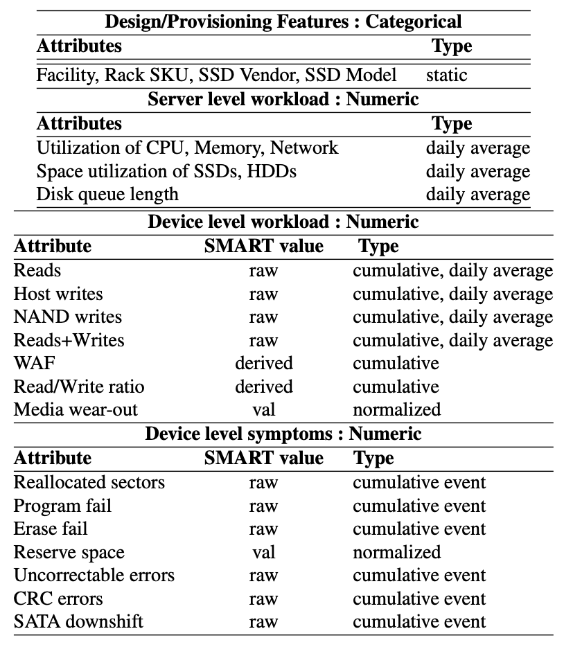
- The table below presents the data collected and used for this study.
- AFR proxies: Annual Replacement/Repairment rate
- Failed Device: We identify an SSD to fail-stop, if the result of some underlying SSD events/failures propagates to the corresponding server, causing it to be shutdown for external (sometimes physical) intervention or investigation. The device will be replaced or repaired subsequently. We refer to a device that fail-stops anytime during our observation window, as a “Failed” device.
- Key Findings:
- The observed Annualized Failure Rate (AFR) in these production datacenters for some models is significantly higher (as much as 70%) than that quoted in SSD specifications, reiterating the need for this kind of field study.
- Four symptoms - Data Errors (Uncorrectable and CRC), Sector Reallocations, Program/Erase Failures and SATA Downshift - experienced by SSDs at the lower levels are the most important (in that order) of those captured by the SMART attributes.
- Even though Uncorrectable Bit Errors in our environment are not as high as in a prior study, it is still at least an order of magnitude higher than the target rates.
- There is a higher likelihood of the symptoms (captured by SMART) preceding SSD failures, with an intense manifestation preventing their survivability beyond a few months. However, our analysis shows that these symptoms are not a sufficient indicator for diagnosing failures.
- Other provisioning (what model? where deployed? etc.) and operational parameters (write rates, write amplifica- tion, etc.) all show some correlation with SSD failures. This motivates the need for not just a relative ordering of their influence (to be useful to a datacenter operator), but also a systematic multi-factor analysis of them all to better answer the what, when and why of SSD failures.
- We use machine learning models and graphical causal models to jointly evaluate the impact of all relevant factors on failures. We show that
- (i) Failed devices can be differentiated from healthy ones with high precision (87%) and recall (71%) using failure signatures from tens of important factors and their threshold values;
- (ii) Top factors used in accurate identification of failed devices include: Failure symptoms of data errors and reallocated sectors, device and server level workload factors such as total NAND writes, total reads and writes, memory utilization, etc.;
- (iii) Devices are more likely to fail in less than a month after their symptoms match failure signatures, but, they tend to survive longer if the failure signature is entirely based on workload factors;
- (iv) Causal analysis suggests that symptoms and the device model have direct impact on failures, while workload factors tend to impact failures via media wear-out.
Alibaba (2019)
- Article Title: Lessons and Actions: What We Learned from 10K SSD-Related Storage System Failures
- Component under Investigation: SSD
- Scale: Around 450,000 SSDs deployed in 7 datacenters of Alibaba
- Data sources:
- At the system level, the daemons monitor BIOS messages, kernel syslogs, and the service-level verification of data integrity. Upon an abnormal event, the daemon reports a failure ticket with the timestamp, the related hardware component, and a log snippet describing the failure. Each failure ticket is tagged based on the component involved. For example, if an SSD appears to be missing from the system, the failure ticket is tagged as ”SSD-related”. If there is no clear hardware component recorded in the logs, the ticket would be tagged as Unknown.
- At the device level, the daemons record SMART attributes on a daily basis, which cover a wide set of device behaviors (e.g., total LBA written, uncorrectable errors).
- Besides the failure tickets and SMART logs, we collect the repair logs of all RASR failures, which are generated by on-site engineers after fixing the failures. For each failure event, the corresponding repair log records the failure symptom, the diagnosis procedure, and the successful fix.
- AFR proxies: Failures that are reported as "SSD-Related" (RASR) by system status monitoring daemons.
- Key Findings:
- "We collect all failure tickets reported as related to hardware components, over 150K tickets in total. The table below shows the distribution of the failure events based on the types of hardware components involved, including CPU, Memory, Network, Motherboard, HDD/SSD, and Unknown."
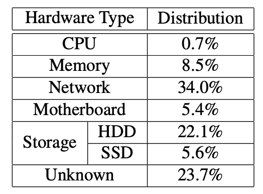
Table: Distribution of failure tickets based on hardware types
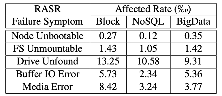
- "We observe that SSDs deployed in one particular datacenter (DC4) experience much more Media Error under the Block Storage service... We find that there are two potential factors."
- First, in DC4, about 27.1% Block service nodes are equipped with 18 SSDs, while in other datacenters less than 5.3% Block service nodes have 18 SSDs (most nodes have 12 SSDs).
- Second, in DC4, nodes for different services are often co-located in the same rack, while in other datacenters a rack is exclusively used for a single service.
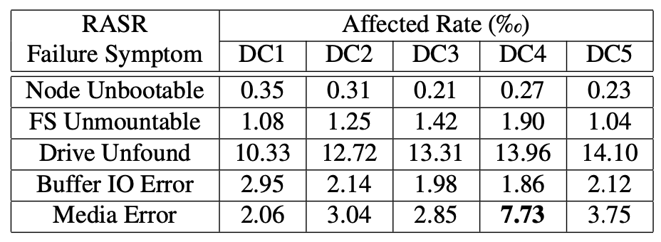
- “We observe that the Block service (2nd column) has the highest affected rates in four out of five types of RASR failures (except Node Unbootable). "
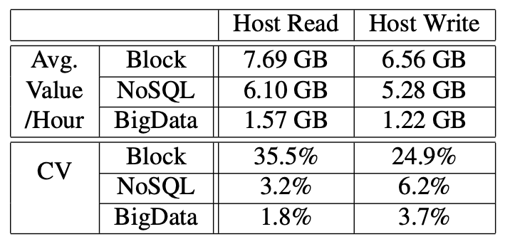
- "We can see that the hourly average value of host read and host write of the Block service are 7.68 GB and 6.56 GB, respectively, which are similar to those of the NoSQL service. However, the Block service has much higher variances for the two metrics (i.e., 35.5% and 24.9%), which implies that the usage of SSDs under this service is much more unbalanced. "
- "We find that ... When an SSD has 17 or more UCRC(Ultra-DMA CRC) errors, it is a strong indication of a faulty interconnection in the target system.
- Note: Ultra-DMA CRC: UDMA (Ultra DMA) stands for Ultra Direct Memory Access. It is a hard drive technology that allows hard drives to communicate directly with memory without relying on the CPU. CRC stands for Cyclic Memory Check, which is a checksum that can detect if data is corrupted. When you combine the two, the Ultra DMA CRC error count indicates problems with the transfer of data between the host and the disk.
4. Conclusions and Recommendations
Through our comprehensive review of existing failure research, it’s evident that nearly all major cloud service providers have embarked on their own failure studies in recent decades, with some conducting multiple investigations.
Research focus has evolved from merely describing failure patterns to uncovering the fundamental causes of key component failures. The data utilized in these studies has grown increasingly diverse, extending beyond mere replacement and fault records to include insights from SMART (Self-Monitoring, Analysis, and Reporting Technology) register and log analyses.
As a leading IDC supply chain service provider, ApexCDS has been conducting failure rate research and analysis for years. We are confident in providing cutting-edge and advanced failure rate analysis and prediction for large-scale IT system.