
Deep Learning Training Algorithm III: Second-Order Optimization Algorithms
In the previous blog post, we have introduced the Gradient-Based Optimization Algorithms, which use the first-order derivatives of the objective function to adjust the model parameters during the training process. However, the first-order methods may suffer from slow convergence, oscillations, and instabilities in some cases, especially for ill-conditioned or non-convex optimization problems.
To address these issues, the Second-Order Optimization Algorithms have been proposed, which utilize the second-order derivatives of the objective function to estimate the curvature and direction of the gradient, and thus may converge faster and more accurately than the first-order methods. In this blog post, we will cover the principles, advantages, and limitations of the Second-Order Optimization Algorithms, as well as several representative examples.
1. Newton's Method
The Newton's Method is the most classical Second-Order Optimization Algorithm, which updates the model parameters by solving a system of linear equations derived from the Hessian matrix of the objective function. Let's break it down to see how it works.
Since the cost functions are not always linear, sometimes we are interested in their second derivative to take the curvature into account. For example, for a function $f: \mathbb{R}^{n} \rightarrow \mathbb{R}$, the derivative with respect to $x_{i}$ of the derivative of $f$ with respect to $x_{j}$ is denoted as $\frac{\partial ^{2}}{\partial x_{i} \partial x_{j}}f$. The second derivative tells us how the first derivative will change as we vary the input.
We can think of the second derivative as measuring curvature. Suppose we have a quadratic function. If such a function has a second derivative of zero, then there is no curvature. It is a perfectly flat line, and its value can be predicted using only the gradient. If the gradient is 1, then we can make a step of size $\epsilon$ along the negative gradient, and the cost function will decrease by $\epsilon$. If the second derivative is positive, the function curves upward, so the cost function can decrease by less than $\epsilon$, which can be illustrated as follows:
When the function has multiple input dimensions, there are many second derivatives. These derivatives can be collected together into a matrix called the Hessian matrix. The Hessian matrix $H(f)(\mathbf{x})$ is defined as
$$\mathbf{H}(f)(\mathbf{x})_{i,j} = \frac{\partial ^2}{\partial x_{i} \partial x_{j}}f(\mathbf{x}).$$
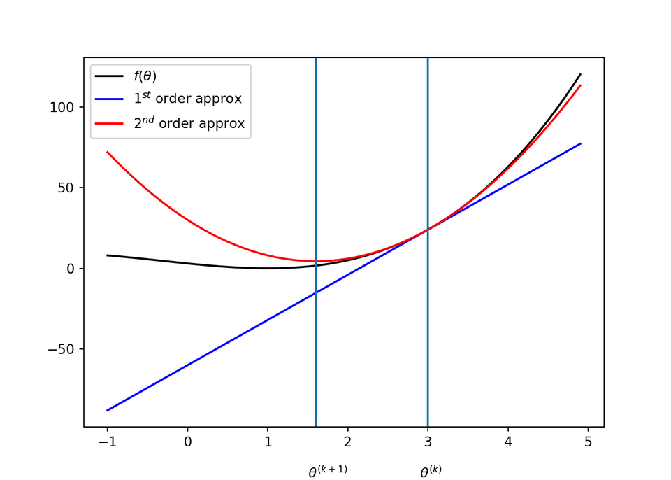
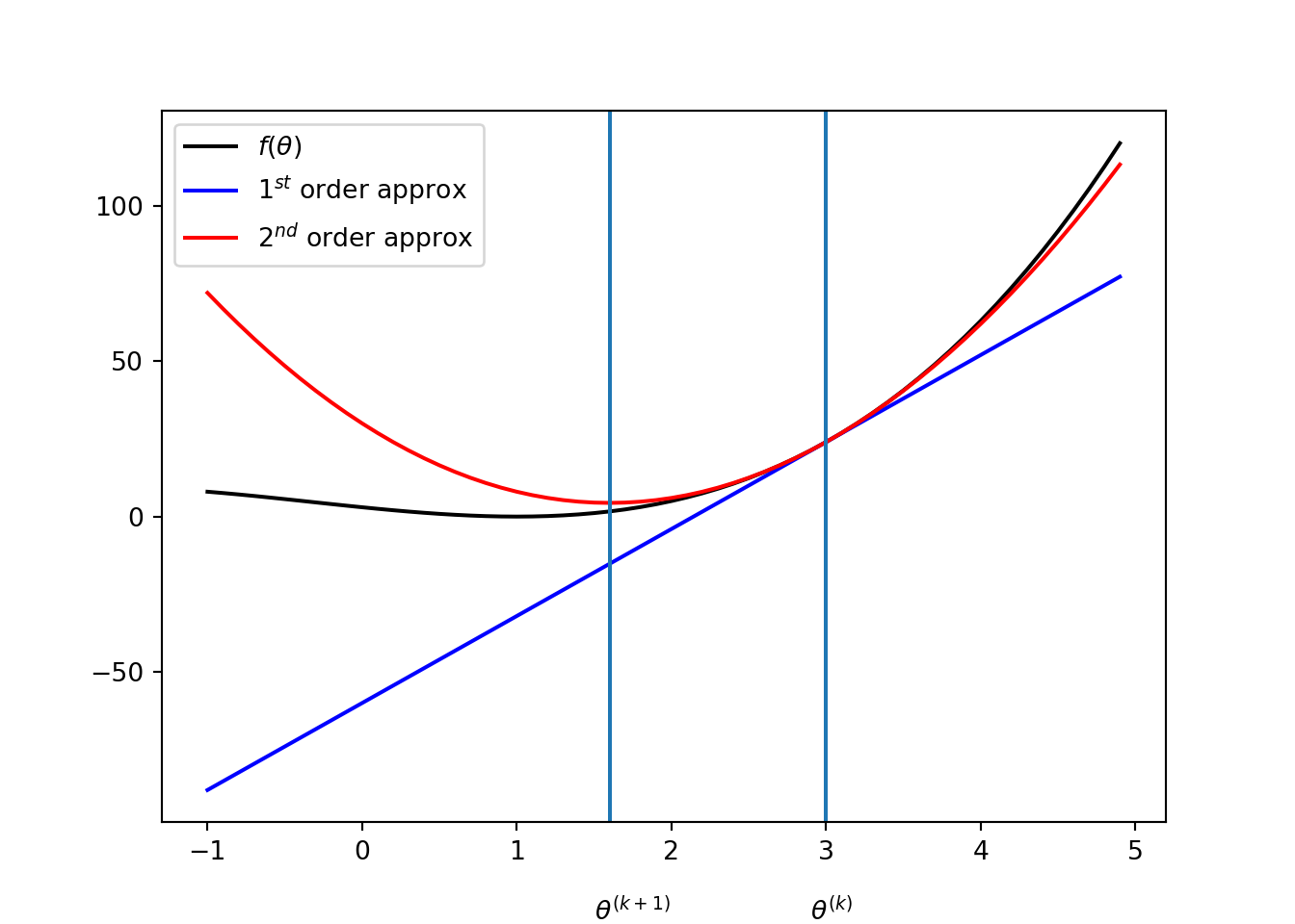
The second derivative can tell us how well we can expect a gradient descent step to perform. We can make a second-order Taylor series approximation to the function $f(\mathbf{x})$ around the current point $\mathbf{x}^{(0)}$:
$$f(\mathbf{x}) \approx f(\mathbf{x}^{(0)}) + (\mathbf{x} - \mathbf{x}^{(0)})^{T} \mathbf{g} + \frac{1}{2}(\mathbf{x} - \mathbf{x}^{(0)})^{T} \mathbf{H} (\mathbf{x} - \mathbf{x}^{(0)})$$
Newton's method is based on using the second-order Taylor series expansion mentioned above. If we solve for the critical point of that function, we obtain
$$\mathbf{x}^{*} = \mathbf{x}^{(0)} - \mathbf{H}(f)(\mathbf{x}^{(0)})^{-1} \nabla_{\mathbf{x}}f(\mathbf{x}^{(0)}) \qquad \qquad (*) $$
When $f$ is a positive definite quadratic function, Newton's method consists of applying equation (*) once to jump to the minimum of the function directly. When $f$ is not truly quadratic but can be locally approximated as a positive definite quadratic, Newton's method consists of applying equation (*) multiple times. Newton's method is only appropriate when the nearby critical point is a minimum, whereas gradient descent is not attracted to saddle points unless the gradient points toward them.
2. L-BFGS
The Newton's Method can converge in a few iterations for well-conditioned convex problems, but may be computationally expensive and unstable for ill-conditioned or non-convex problems. To address these issues, various Quasi-Newton Methods have been proposed, which approximate the Hessian matrix using limited memory or rank-one updates, and thus reduce the computational cost and improve the stability of the algorithm.
One of the most popular Quasi-Newton Methods is the Limited-Memory BFGS (L-BFGS), which stores a limited number of past gradients and updates the inverse Hessian approximation using a rank-one update scheme. The L-BFGS is efficient, stable, and widely used in many deep learning applications, such as image recognition, natural language processing, and speech synthesis. Let take a closer look at the Broyden-Fletcher-Goldfarb-Shanno (BFGS) altorithm first.

Broyden-Fletcher-Goldfarb-Shanno (BFGS)
The BFGS attempts to bring some of the advantages of Newton's method without the computational burden. Recall that Newton's update is given by
$$\mathbf{x}^{*} = \mathbf{x}^{(0)} - \mathbf{H}(f)(\mathbf{x}^{(0)})^{-1} \nabla_{\mathbf{x}}f(\mathbf{x}^{(0)}) $$
where $\mathbf{H}$ is the Hessian matrix respect of $\mathbf{x}$ evaluated at $\mathbf{x}^{(0)}$. The primary computational difficulty in applying Newton's update is the calculation of the inverse Hession $\mathbf{H}^{-1}$. The approach adopted by quasi-Newton methods is to approximate the inverse with a matrix $\mathbf{M}_{t}$ that is iteratively refined by low-rank updates to become a better approximation of $\mathbf{H}^{-1}$.
Once the inverse Hessian approximation $\mathbf{M}_{t}$ is updated, the direction of descent $\mathbf{\rho}_{t}$ is determined by $\mathbf{\rho}_{t} = \mathbf{M}_{t}\mathbf{g}_{t}$. A line search is performed in this direction to determine the size of the step, $\epsilon^{*}$, taken in this direction. The final update to the parameters is given by
$$\mathbf{x}_{t+1} = \mathbf{x}_{t} + \epsilon^{*}\mathbf{\rho}_{t}$$
The BFGS algorithm iterates a series of line serches with the direction incorporating second-order information. However, it is not heavily dependent on the line search finding a point very close to the true minimum along the line. On the other hand, the BFGS algorithm must store the inverse Hessian matrix $\mathbf{M}$, that requires $\mathcal{O}(n^2)$ memory, making BFGS impractical for most modern deep learning models that typically have millions of parameters.
Limited Memory BFGS (L-BFGS)
The memory costs of the BFGS algorithm can be significantly decreased by avoiding storing the complete inverse Hessian approximation $\mathbf{M}$. The L-BFGS algorithm computes the approximation $\mathbf{M}$ using the same method as the BFGS algorithm but beginning with the assumption that $\mathbf{M}^{t-1}$ is the identity matrix, rather than storing the approximation from one step to the next. The L-BFGS strategy with no storage described here can be generalized to include more information about the Hessian by storing some of the vectors used to update $\mathbf{M}$ at each time step, which costs only $\mathcal{O}(n)$ per step.
3. Levenberg-Marquadt Algorithms (LMA)
Levenberg-Marquardt Algorithm combines the advantages of the first-order and second-order methods by using a damping parameter to balance between the gradient and Hessian information.
If the fitting function is denoted by $\hat{y}(t; \mathbf{p})$ and $m$ data points denoted by $(t_{i}, y_{i})$, then the squared error can be written as:
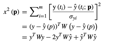
where the measurement error of $y(t_i)$, i.e., $\sigma_{yi}$ is the inverse of the weighting matrix $W_{ii}$
The gradient descent of the squared error function in relation to the $n$ parameters can be denoted as:
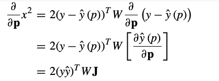
where $\mathbf{J}$ is the Jacobian matrix. So the update in the direction of the steepest gradient descent can be written as
$$h_{gd} = \alpha \mathbf{J}^{T} W(y-\hat{y})$$
The equation for the Gauss-Newton method update ($h_{gn}$) is as follows
$$[\mathbf{J}^{T}W\mathbf{J}] = \mathbf{J}^{T}W(y-\hat{y})$$
Levenberg's contribution is to replace this equation by a "damped version". The Levenberg-Marquardt update ($h_{lm}$) is generated by combining gradient descent and Gauss-Newton methods resulting in the equation below:
$$[\mathbf{J}^{T}W\mathbf{J} + \lambda diag(\mathbf{J}^{T}W\mathbf{J})]h_{lm} = \mathbf{J}^{T}W(y-\hat{y})$$
The LMA is used in many software applications for solving generic curve-fitting and optimization problems. It often converges faster than first-order methods. However, like other iterative optimization algorithms, the LMA finds only a local minimum, which is not necessarily the global mininums.
In the next blog post, we will cover some similar shortcomings of training algorithms, namely, the vanishing and exploding gradients, local minima, flat regions, and so on. Stay tuned!