Deep Learning Training Algorithms II: Gradient-Based Optimization Algorithms

Introduction

Deep learning models are powerful tools for solving complex problems in a variety of domains, from image and speech recognition to natural language processing and robotics. At the heart of deep learning lies the concept of training, which involves feeding a model with large amounts of data and adjusting its parameters to minimize the difference between the predicted and true values.

Gradient-based optimization algorithms are the most commonly used class of training algorithms in deep learning, as they are efficient, scalable, and easy to implement. By iteratively adjusting the model parameters in the direction of the steepest descent of the loss function, these algorithms can find an optimal solution that minimizes the training error.

In this post, we will provide an overview of gradient-based optimization algorithms, including their variants and extensions, and discuss their pros and cons in different scenarios.

2. Gradient-Based Optimization Algorithms

Gradient-based optimization algorithms are a family of iterative methods that use the gradient of the loss function to update the model parameters in the direction of the steepest descent.

The basic idea is to compute the gradient of the loss function with respect to each parameter and adjust its value by a small amount proportional to the negative gradient, with the goal of reducing the loss function over time. The following are some of the most commonly used gradient-based optimization algorithms in deep learning:

• Batch gradient descent: This algorithm updates the model parameters after computing the gradient of the loss function over the entire training set. Although it can lead to accurate convergence in some cases, it can also be computationally expensive and slow to converge.

• Stochastic gradient descent (SGD): This algorithm updates the model parameters after computing the gradient of the loss function on a single randomly selected example from the training set. It can be faster and more efficient than batch gradient descent, but it can also be more noisy and prone to getting stuck in local minima.

• Mini-batch SGD: This algorithm updates the model parameters after computing the gradient of the loss function on a small subset of examples (e.g., 32, 64, or 128) from the training set. It combines the advantages of batch gradient descent and SGD, allowing for a compromise between accuracy and efficiency.

• Momentum: This algorithm adds a fraction of the previous update to the current update, in order to accelerate convergence and dampen oscillations. It can be seen as a way to add inertia to the optimization process, allowing it to escape local minima and smooth out noisy gradients.

• Adaptive learning rate algorithms: These algorithms adjust the learning rate of each parameter based on its history of gradients, in order to speed up convergence and improve stability. Examples include AdaGrad, which adapts the learning rate for each parameter based on the sum of the squares of the past gradients, and RMSprop and Adam, which use exponentially decaying averages of the past gradients and their squares to scale the learning rate.

Now, we will walk through some commonly used gradient optimization algorithms.

2.1. Gradient Descent

Gradient descent (GD) is the underlying idea in most of machine learning and deep learning algorithms. It is based on the concept of Newton's Algorithm for finding the roots of a 2D funcition. To achieve this, we randomly pick a point in the curve and slide to the right or left along the $x$-axis based on negative or positive value of the derivative or slope of the function at the chosen point until the value of the $y$-axis, i.e., function or f(x) becomes zero.

The same idea is used in gradient descent, where we traverse or descend along a certain path in a multi-dimentional weight space if the cost function keeps decreasing and stop once the error rate ceases to decrease. Newton's method is prone to getting stuck in local minima (shown below) if the derivative of the function at the current point is zero.

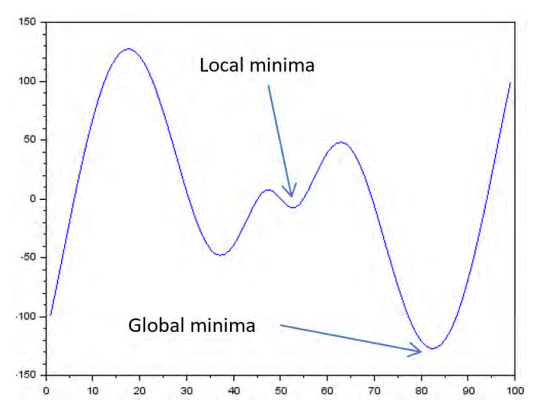
Likewise, this risk is also present when using gradient descent on a non-convex function. In fact, the impact is amplified in the multi-dimensional and multi-layer landscape of DNN and it result in a sub-optimal set of weights. Cost function is one half the sqare of the difference between the desired output minus the current output as shown below.

$$C = \frac{1}{2} (y_{expected} - y_{actual})^{2}$$

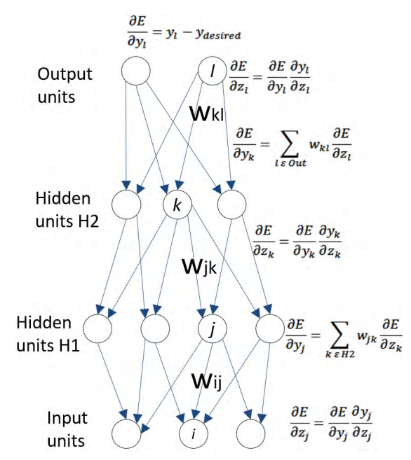
Backpropagation methodology uses gradient descent. In backpropagation, chain rule and partial derivatives are employed to determine error delta for any change in the value of each weight. The individual weights are then adjusted to reduce the cost funtion after multi-dimensional (multi-weight) landscape of weight values. We process through all the samples in the training dataset before applying the updates to the weights. This process repeated until objective doesn't reduce any further.

The figure below shows the error derivatives in relation to outputs in each hidden layer, which is the weighted summation of above layer. E.g., when $\partial E / \partial z_{k}$ is calculated, the partial error derivative with respect to $w_{jk}$ to is equal to $y_{j} \partial E / \partial z_{k}$.

2.2 Stochastic Gradient Descent

Stochastic Gradient Descent (SGD) is the most common variation and implementation of gradient descent.In gradient descent, we process through all the samples in the training dataset before applying the updates to the weights. While batch before applying the updates to the weights. While in SGD, updates are applied after running through a mini-batch of $n$ number of samples. In other words, when used to minimize the cost function, as standard (or "batch") gradient descent method would perform the following iterations:

$$w:= w - \eta \nabla C(w) = w - \frac{\eta}{n} \sum_{n=1}^{n} \nabla C_{i}(w)$$

where $C$ is the cost function and $\eta$ is the learning rate.

In stochastic (or "on-line") gradient descent, the true gradient of the cost function $C$ is approximated by a gradient at a single sample:

$$w := w - \eta \nabla C_{i}(w)$$

Since we are updating the weights more freshently in SGD than in GD, we can converge towards global minimum each faster.

A compromise between computing the true gradient and the gradient at a single sample is to compute the gradient against more than one training sample (called a "mini-batch") at each step. This can perform significantly better than "true" stochastic gradient descent described, because the code can make use of vectorization libraries rather than computing each step separately. It may also result in smoother convergence, as the gradient computed at each step is averaged over more training sample.

2.3. Extensions and Variants

Many improvements on the basic (stochastic) gradient decent algorithm have been proposed and used. In particular, in machine learning, the setting of hyperparameter learning rate $\eta$ can be tricky. Large learning rate may result in diverging, however, small learning rate can drag down the converging speed. Practical guidance on choosing the step size in several variants of SGD is given by the researchers.

Implicit Updated Stochastic Gradient Descent (ISGD)

By considering implicit updates whereby the stochastic gradient is evaluated at the next iterate rather than the current one:

$$w^{new} := w^{old} - \eta \nabla C_{i}(w^{new})$$

This equation is implicit since $w^{new}$ appears on both sides of the equation.

As an example, consider least squares with features $x_{1}, \ldots, x_{n} \in \mathbb{R}^{p}$ and observations $y_{1}, \ldots, y_{n} \in \mathbb{R}$. We wish to solve:

$$\min_{w} \sum_{j=1}^{n}(y_{j} - x_{j}^{'}\cdot w)^{2}$$

Classical stochastic gradient descent proceeds as follows:

$$w^{new} = w^{old} + \eta(y_{i} - x_{i}^{'}\cdot w^{old})x_{i} $$

where $i$ is uniformly sampled between 1 and $n$. Although theoretical convergence of this procedure can be garranteed under relatively mild assumptions, in practice the procedure can be quite unstable. In particular, when $\eta$ is misspecified so that $I-\eta x_{i}x_{i}^{'}$ has large absolute eigenvalues with high probability, the procedure may diverge numerically within a few iterations. In contrast, ISGD can be solved in closed-form as:

$$w^{new} = w^{old} + \frac{\eta}{1+\eta || x_{i} || ^{2}}(y_{i} - x_{i}^{'}\cdot w^{old})x_{i} $$

This procedure will remain numerically stable virtually for all $\eta$ as the learning rate is now normalized. Such comparison between classical and implicit stochastic gradient descent in the least squares problem is very similar to the comparison between least mean squares and normalized least mean squares filter.

Even though a closed-form solution for ISGD is only possible in least squares, the procedure can be efficiently implemented in a wide range of models.

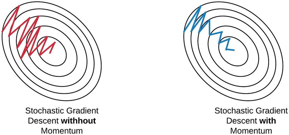
Momentum

Further proposals include the momentum method or the heavy ball method, which in ML context appeared in Rumelhart, Hinton and Williams' paper on backpropagation learning and borrowed the idea from Soviet mathematician Boris Polyak's 1964 article on solving functional equations. Stochastic gradient descent with momentum remembers the update $\Delta w$ as each iteration, and determines the next update as a linear conbination of the gradient and the previous update:

$$w := w - \eta \nabla C_{i}(w) + \alpha \Delta w$$

where $\alpha$ is an exponential decay factor between $0$ and $1$ that determines the relative contribution of the current gradient and earlier gradients to the weight change.

By using the concept of momentum in physics, the momentum algorithm helps prevent costly descent in the wrong direction as illustrated below:

AdaGrad

AdaGrad (for adaptive gradient algorithm) is a modified stochastic gradient descent algorithm with per-parameter learning rate. Informally, this increases the learning rate for sparser parameters and decreases the learning rate for ones that are less sparse. This strategy often improves convergence performance over standard stochastic gradient descent in settings where data is sparse and sparse parameters are more informative.

It still has a base learning rate $\eta$, but this is multifplied with the elements of a vector ${\G_{j,j}}$, which is the diagonal of the outer product matrix

$$G = \sum_{\tau = 1}^{t} g_{\tau}g_{\tau}^{T}$$

where $g_{\tau} = \nabla C_{i}(w)$, the gradient, at iteration $\tau$. The diagonal is given by

$$G_{j,j} = \sum_{\tau = 1}^{t} g_{\tau, j}^{2}$$

This vector essentially stores a historical sum of gradient squares by dimension and is updated after every iteration. The formula for an update is now

$$w := w - \eta \diag (G)^{-\frac{1}{2}} \odot g$$

or, written as per-parameter updates,

$$w_{j} := w_{j} - \frac{\eta}{\sqrt{G_{j,j}}}g_{j}$$

Each ${G_{j,j}}$ gives rise to a scaling factor for the learning rate that applies to a single parameter $w_{j}$.

RMSProp

RMSProp is a method invented by Geoffrey Hinton in 2012 in which the learning rate is, like in Adagrad, adapted for each of the parameters. The idea is to divide the learning rate for a weight by a running average of the magnitudes of recent gradients for that weight.

First the running average is calculated in terms of means square,

$$v(w,t) := \gamma v(w, t-1) + (1 - \gamma) (\nabla C_{i}(w))^{2}$$

where, $\gamma$ is the forgetting factor. The concept of storing the historical gradient as sum of squares is borrowed Adagrad, but "forgetting" is introduced to solve AdaGrad's diminishing learning rates in non-convex problems by gradually decreasing the influence of old data.

And the parameters are updated as,

$$w := w - frac{\eta}{\sqrt{v(w,t)}} \nabla Q_{i}(w)$$

RMSProp has shown good adaptation of learning rate in different applications.

Adam

Adam (short for Adaptive Moment Estimation) is a 2014 update to the RMSProp optimizer combining it with the main feature of the Momentum method. In this optimization algorithm, running averages with exponential forgetting of both the gradients and the second moments of the gradients are used. Given parameters $w^{(t)}$ and a cost function $C^{(t)}$, where $t$ indexes the current training iteration, Adam's parameter update is given by:

$m_{w}^{(t+1)} \leftarrow \beta_{1}m_{w}^{(t)} + (1 - \beta_{1}) \nabla_{w}C^{(t)}$

$v_{w}^{(t+1)} \leftarrow \beta_{2}v_{w}^{(t)} + (1 - \beta_{2}) (\nabla_{w}C^{(t)})^{2}$

$\hat{m}_{w} = \frac{m_{w}^{(t+1)}}{1 - \beta_{1}^{t}}$

$\hat{v}_{w} = \frac{v_{w}^{(t+1)}}{1 - \beta_{2}^{t}}$

$w^{(t+1)} \leftarrow w^{(t)} - \eta \frac{\hat{m}_{w}}{\sqrt{\hat{v}_{w}}+\epsilon}$

where $\epsilon$ is a small scalar used to prevent division by $0$, and $\beta_{1}$ and $\beta_{2}$ are the forgetting factors for gradients and second moments of gradients, respectively.

The profound influence of this algorithm inspired multiple newer, second-order information (for example, Powerpropagation and AdaSqrt). However, the most commonly used variants are AdaMax, which genearalizes Adam using the infinity norm, and AMSGrad, which addresses convergence problems from Adam by using maximum of past squared gradients instead of the exponential average.

3. Conclusion

In this blog post, we have covered the first category of deep learning training algorithms, namely, the Gradient-Based Optimization Algorithms. We have discussed their general principles, advantages, and limitations, as well as several representative examples, including the Stochastic Gradient Descent (SGD), the Batch Gradient Descent (BGD), the Mini-Batch Gradient Descent (MBGD), the Momentum, the AdaGrad, the RMSprop, and the Adam.

It is worth noting that the Gradient-Based Optimization Algorithms are the most widely used training algorithms in deep learning due to their simplicity, efficiency, and scalability. They are particularly effective for convex optimization problems, but may encounter difficulties in non-convex optimization problems, such as local minima, saddle points, and plateaus. Therefore, it is important to choose appropriate learning rates, batch sizes, and momentum parameters, and to apply regularization techniques such as L1/L2 regularization and dropout to avoid overfitting and improve generalization performance.

In the next blog post, we will cover the second category of deep learning training algorithms, namely, the Second-Order Optimization Algorithms. These algorithms utilize the second-order derivatives of the objective function to estimate the curvature and direction of the gradient, and thus may converge faster and more accurately than the first-order methods. However, they are computationally more expensive and may suffer from numerical stability issues. We will discuss their principles, advantages, and limitations, as well as several representative examples, including the Newton's Method, the Quasi-Newton Methods, and the Limited-Memory BFGS (L-BFGS). Stay tuned!