Review of Deep Learning Algorithms and Architectures II: CNN Architectures
A Deep neural network consists of several layers of nodes. Different architectures have been developed to solve problems in different domains and have their own applications. For instance, CNN is often used in computer vision and image recognition, and RNN is commonly used in time series analysis and forecasting. Below are four of the most common architectures of deep neural networks.
- Convolution Neural Network (CNN)
- Autoencoder
- Restricted Bolzmann Machine (RBM)
- Long Short-Term Memory (LSTM)
In this post, we will mainly explain the architecture of CNN.
Introduction to Convolution Neural Network (CNN)
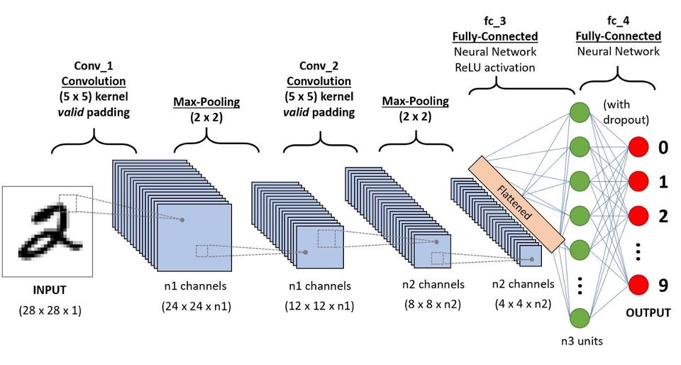
CNN is based on the human visual cortex and is the neural network of choice for computer vision (image recognition) and video recognition. It is also used in other areas such as NLP, drug discovery, etc. As shown in the figure below, a CNN consists of a series of convolutional and pooling layers followed by a fully connected layer and normalizing layer.
Convolutional Layer
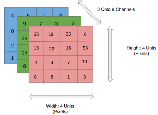
First, an RGB image is separated by its three color planes - Red, Green, and Blue. Like this
Then we can use the Kernel/Filter matrix to convolute an image input into a lower dimensional convolved feature.
In the above demonstration, the green section resembles the $5\times 5 \times 1$ input image. For each $3\times 3 \times 1$ submatrix of the input image, we multiply it with the Kernel/Filter matrix, which is represented in yellow. Then we obtain an output convolved feature matrix, which is $3\times 3 \times 1$ in pink.
The Kernel shifts 9 times because of Stride Length = 1 (Non-strided), every time performing a matrix multiplication operation between K and the portion P of the image over which the kernel is hovering.
The filter moves to the right with a certain Stride Value untill it parses the complete width. Moving on, it hops down to the far left of the image with the same Stride Value and repeats the process until the entire image is traversed.
In the case of images with multiple channels (e.g. RGB), the Kernel has the same depth as that of the input image. For instance, in our previous example, the Kernel has three layers illustrated in the figure below.
Then the sub matrice extracted from the color image are multiplied by their corresponding Kernels and all the results are summed with the bias to give us a squashed one-depth channel Convoluted Feature Output.
The objective of the Convolution Operation is to extract the high-level features such as edges, from the input image. ConvNets need not be limited to only one Convolutional Layer. In the figure illustrating digit recognition, there are two convolutional layers.
Conventionally, the first ConvLayer is responsible for capturing the low-level features such as edges, color, gradient orientation, etc. With more ConvLayers, the architecture adapts to the High-Level features as well, giving us a network, which has a wholesome understanding of images similar to that of the human being.
There are two types of results to the operation -- one in which the convolved feature is reduced in dimensionality as compared to the input, and the other in which the dimensionality is either increased or remains the same. This is done by applying Valid Padding in case of the former, or Same Padding in the case of the latter.
Taking the same example, in Same Padding, we augment the $5\times 5 \times 1$ image into a $6\times 6 \times 1$ image and then apply the $3\times 3 \times 1$ Kernel over it, we find that the convolved matrix turns out to be of dimension $5\times 5 \times 1$. Hence the name -- Same Padding.
On the other hand, if we perform the same operation without padding, we are presented with a matrix that has dimensions of the Kernel ($3\times 3 \times 1$) itself -- Valid Padding.
Pooling Layer
Similar to the Convolutional Layer, the Pooling Layer is responsible for reducing the spatial size of the Convolved Feature. This is to decrease the computational power required to process the data through dimensional reduction. Furthermore, it is useful for extracting dominant features which are rotational and translational invariant, thus maintaining the process of effectively training the model.
There are two types of Pooling: Max Pooling and Average Pooling.
-
Max Pooling returns the maximum value from the portion of the image covered by the Kernel.
-
Average Pooling returns the average of all the values from the portion of the image covered by the Kernel.
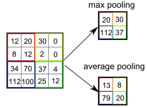
Max Pooling also performs as a Noise Suppressant. It discards the noisy activations altogether and also performs de-noising along with dimensionality reduction. On the other hand, Average Pooling simply performs dimensionality reduction as a noise suppressing mechanism. Hence, sometimes Max Pooling performs a lot better than Average Pooling.
The Convolutional Layer and the Pooling Layer, together form the ith layer of a Convolutional Neural Network. Depending on the complexities of the problem, the number of such layers may be increased for capturing low-level details even further, but at the cost of more computational power.
After going through the above process, we have successfully enabled the model to understand the features. Moving on, we are going to flatten the final output and feed it to a regular Neural Network for classification purposes.
Fully Connected Layer
Adding a Fully-Connected Layer is a (usually) cheap way of learning non-linear combinations of the high-level features as represented by the output of the convolutional layer. The Fully-Connected layer is learning a possibly non-linear function in that space.
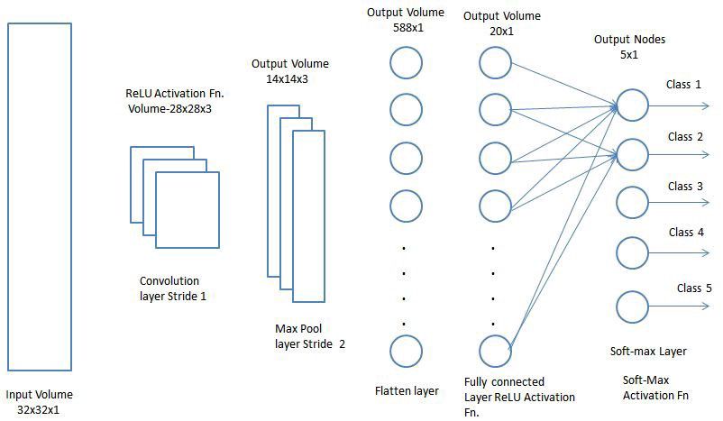
Now that we have converted our input image into a suitable form for our Multi-Level Perceptron, we shall flatten the image into a column vector. The flattened output is sed to a feed-forward neural network and backpropagation applied to every iteration of training. Over a series of epochs, the model is able to distinguish between dominating and certain low-level features in images and classify them using the Softmax Classification technique.
Here are some well-known variations and implementations of the CNN architecture.
- AlexNet: CNN developed to run on Nvidia parallel computing platform to support GPUs.
- Inception: Deep CNN developed by Google
- ResNet: Very deep Residual network developed by Microsoft.
- VGG: Very deep CNN developed for large-scale image recognition.
- DCGAN: Deep convolutional generative adversarial networks, which is used in unsupervised learning of hierarchy of feature representations in input objects.
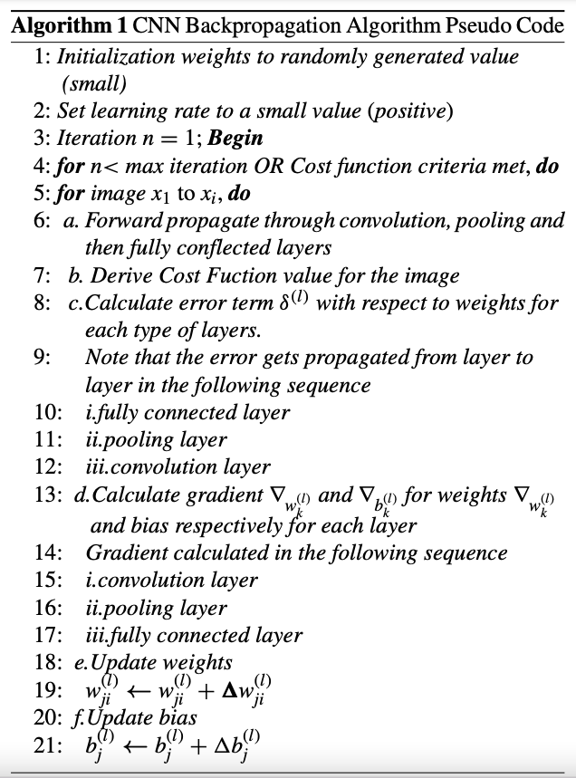
Appendix: CNN Backpropagation Algorithm Pseudo Code
In most cases, backpropagation is used solely for training all parameters (weights and biases) in CNN. Here is a brief description of the algorithm. The cost function with respect to individual training example $(x,y)$ in hidden layers can be defined as
$$J(W, b; x, y) = \frac{1}{2} |h_{w,b}(x) - y|$$
The equation for error term $\delta$ for layer $l$ is given by
$$\delta ^{(l)} = ((W^{(l)})^{T} \delta^{(l+1)}\cdot f'(z^{(l)}))$$
where $\delta^{(l+1)}$ is the error for $(l+1)$th layer of a network whose cost function is $J(W, b; x, y)\cdot f'(z^{(l)})$ represents the derivate of the activation function.
$$\nabla_{w^{(l)}}J(W, b; x, y) = \delta^{(l+1)}(a^{(l+1)})^{T}$$
$$\nabla_{b^{(l)}}J(W, b; x, y) = \delta^{(l+1)}$$
where $a$ is the input, such that $a^{(1)}$ is the input for 1st layer and $a^{(l)}$ is the input for $l$th layer.
Error for pooling layer can be calculated as:
$$\delta_{k} ^{(l)} = pre-pooling ((W_{k}^{(l)})^{T} \delta_{k}^{(l+1)}\cdot f'(z_{k}^{(l)}))$$
where $k$ represents the filter number in the layer. In the pooling layer, the error has to be cascaded in the opposite direction, e.g., where pooling is used. And finally, here is the gradient w.r.t feature maps:
$$\nabla_{w_{k}^{(l)}}J(W, b; x, y) = \sum_{i-1}^{(l)} (a_{i}^{(l)}) * \text{rot90} ( \delta_{k}^{(l+1)}, 2 )$$
$$\nabla_{b_{k}^{(l)}}J(W, b; x, y) = \sum_{a,b}(\delta_{k}^{(l+1)}) {a,b}$$
where $a^{(l)}$ is the input to the $l$th layer, and $a(1)$ is the input image. The operation $(a_{i}^{(l)})∗\delta_{k}^{(l+1)}$ is the “valid” convolution between $i$th input in the $l$th layer and the error w.r.t. the $k$th filter.
Algorithm 1 below represents a high-level description and flow of the backpropagation algorithm as used in a CNN as it goes through multiple epochs until either the maximum iterations are reached or the cost function target is met.