Review of Deep Learning Algorithms and Architectures I: A Brief Introduction

Introduction

Neural Network is a machine learning technique that is inspired by and resembles the human nervous system and the structure of the brain. It consists of processing units organized in input, hidden and output layers. The nodes or units in each layer are connected to nodes in adjacent layers. Each connection has a weight value.

1. The inputs are multiplied by the respective weights and summed at each unit.
2. The sum then undergoes a transformation based on the activation function.
3. The output of the function is then fed as input to the subsequent unit in the next layer.
4. The result of the final output layer is used as the solution for the problem.

Background

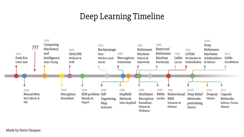
In 1957, Frank Rosenblatt created the perceptron, the first prototype of what we now know as a neural network. It had two layers of processing units that could recognize simple patterns.

Instead of undergoing more research and development, neural networks entered a dark phase of its history in 1969, when professors and MIT demonstrated that it couldn't even learn a simple XOR function.

In addition, there was another finding that particularly dampened the motivation for DNN. The universal approximation theorem showed that a single hidden layer was able to solve any continuous problem. It was mathematically proven as well, which further questioned the validity of DNN.

It was not only the universal approximation theorem that held back the progress of DNN. Back then, we didn't have a way to train a DNN either. These factors prolonged the so-called AI winter, i.e., a phase in the history of AI where it didn't get much funding and interest, and as a result, didn't advance much either.

A breakthrough in DNN occurred with the advent of backpropagation learning algorithm. It was proposed in the 1970s but it wasn't until mid-1980s that it was fully understood and applied to neural networks. The self-directed learning was made possible with a deeper understanding and application of backpropagation algorithm. The automation of feature extractors is what differentiates a DNNs from earlier generation machine learning techniques.

DNN is a type of neutral modeled as a multilayer perceptron (MLP) that is trained with algorithms to learn representations from data sets without any manual design of feature extractors.

As the name Deep Learning suggests, it consists of higher or deeper number of processing layers, which contrasts with shallow learning model with fewer layers of units. The shift from shallow to deep learning has allowed for more complex and non-linear functions to be mapped, as they cannot be efficiently mapped with shallow architectures.

The boom in deep learning also benefits from the proliferation of cheaper processing units such as the general-purpose graphic processing unit (GPGPU) and large volume of data set (big data) to train from. While GPGPUs are less powerful than CPUs, the number of parallel processing cores in them outnumber CPU cores by orders of magnitude.

Classification of Neural Network

Neural Network can be classified into the following different types.

1. Feedforward Neural Network
2. Recurrent Neural Network
3. Radial Basis Function Neural Network
4. Kohonen Self Organizing Neural Network
5. Modular Neural Network

Feedforward Neural Network

In a feedforward neural network, information flows in just one direction from input to output layer. They do NOT form any circles or loopbacks.

The figure below shows a particular type of implementation of a multilayer feedforward neural network with values and functions computed along the forward pass path.

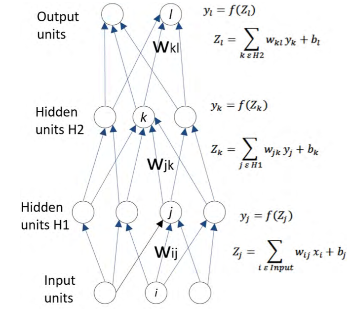
$Z$ is the weighted sum of the inputs and $y$ represents the non-linear activation function $f$ of $Z$ at each layer. $W$ represents the weights between the two units in the adjoining layers indicated by subscript letters and b represents the bias value of the unit.

Recurrent Neural Network

Unlike feedforward neutral networks, the processing units in RNN form a cycle. The output of a layer becomes the input to the next layer, which is typically the only layer in the network, thus the output of the layer becomes an input to itself forming a feedback loop.

This allows the network to have memory about the previous states and use that to influence the current output. One significant outcome of this difference is that unlike feedforward neural network, RNN can take a sequence of inputs and generate a sequence of output values as well, rendering it very useful for applications that require processing sequence of time phased input data like speech recognition, frame-by-frame video classification, etc.

The figure below demonstrates the unrolling of a RNN in time.

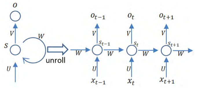
Here is the mathematical explanation of the diagram: $x_{t}$ represents the input at time $t$. $U, V$ and $W$ are the learned parameters that are shared by all steps. $O_{t}$ is the output at time $t$. $S_{t}$ represents the state at time $t$ and can be computed as follows, where $f$ is the activation function.

$$S_{t} = f(U\cdot x_{t} + W \cdot s_{t-1})$$

Radial Basis Function Neural Network

Radial Basis Function (RBF) neural network is used in classification, function approximation, time series prediction problems, etc. It consists of input, hidden and output layers. The hidden layer includes a radial basis function (implemented as Gaussian function) and each node represents a cluster center.

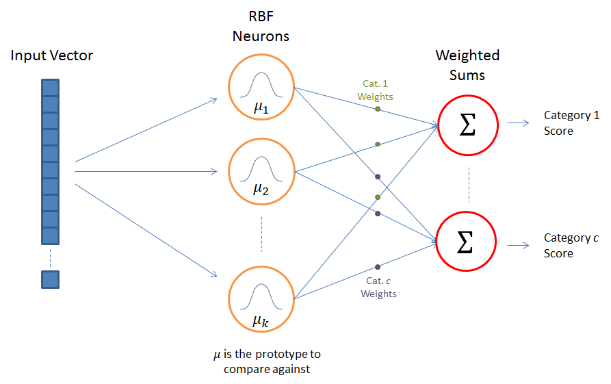
The network learns to designate the input to a center and the output layer combines the outputs of the radial basis function and weight parameters to perform classification or inference.

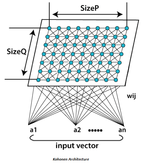
Kohonen Self-organizing Neural Network

Kohonen self-organizing neural network self organizes the network model into the input data using unsupervised learning. It consists of two fully connected layers, i.e., input layer and output layer. The output layer is organized as a two-dimensional grid. There is no activation function and the weights represent the attributes (position) of the output layer node.

The Euclidian distance between the input data and each oupput layer node with respect to the weights are calculated. The weights of the closest node and its neighbors from the input data are updated to bring them closer to the input data with the formula below

$$w_{i}(t+1) = w_{i}(t) + \alpha(t)\eta_{j\star i}(x(t) - w_{i}(t))$$

where $x(t)$ is the input data at time $t$, $w_{i}(t)$ is the $i$th weigh at time $t$ and $\eta_{j\star i}$ is the neighborhood function between the $i$th and $j$th nodes.

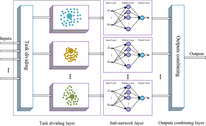
Modular Neural Network

Modular neural network breaks down the large network into smaller independent neural network modules. The smaller networks perform specific tasks which are later combined as part of a single output of the entire network.

DNNs are implemented in the following popular ways:

1. Sparse Autoencoders
2. Convolution Neural Networks (CNNs)
3. Restricted Boltzmann Machines (RBMs)
4. Long Short-Term Memory (LSTM)

Autoencoders are neural networks that learn features or encoding from a given dataset in order to perform dimensionality reduction. Sparse Autoencoder is a variation of Autoencoders, where some of the units output a value close to zero or are inactive and do not fire. Deep CNN uses multiple layers of unit collections that interact with the input and result in desired feature extraction. CNN finds its application in image recognition, recommender systems and NLP. RBM is used to learn probability distribution within the data set.

All these networks use backpropagation for training. Backpropagation uses gradient descent for error reduction, by adjusting the weights based on the partial derivative of the error with respect to each weight.

Neural Network models can also be divided into the following two distinct categories:

1. Discriminative
2. Generative

Discriminative model is a bottom-up approach in which data flows from input layer via the hidden layers to the output layer. They are used in supervised training for problems like classification and regression. Generative models on the other hand are top-down and data flows in the opposite direction. They are used in unsupervised pre-training and probabilistic distribution problems. If the input $x$ and corresponding label $y$ are given, a discriminative model learns the probability distribution $p(y|x)$, i.e., the probability of $y$ given $x$ directly, whereas a generative model learns the joint probability of $p(x, y)$, from which $P(y|x)$ can be predicted. In general whenever labeled data is available discriminative approaches are undertaken as they provide effective training, and when labeled data is not available generative approach can be taken.

Training can be broadly categorized into three types:

1. Supervised
2. Unsupervised
3. Semi-supervised

There is no clear consensus on whether supervised learning is better than unsupervised learning. Both have their merits and use cases.

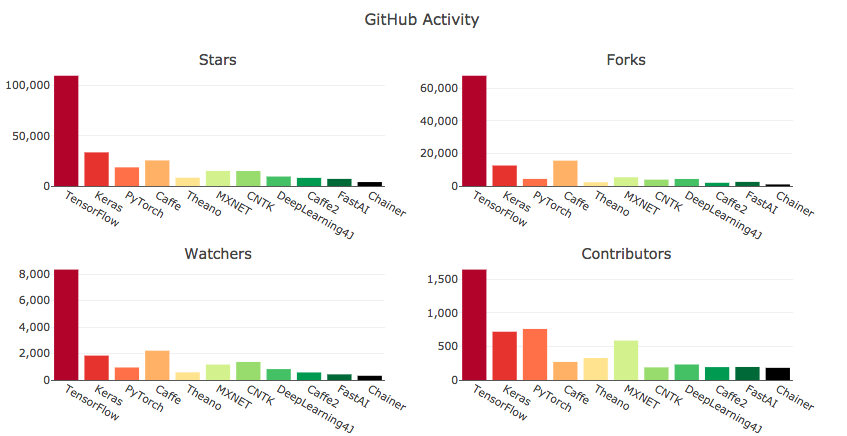
Along with different types of training, algorithms and architecture, we also have different machine learning frameworks and libraries that have made training models easier.

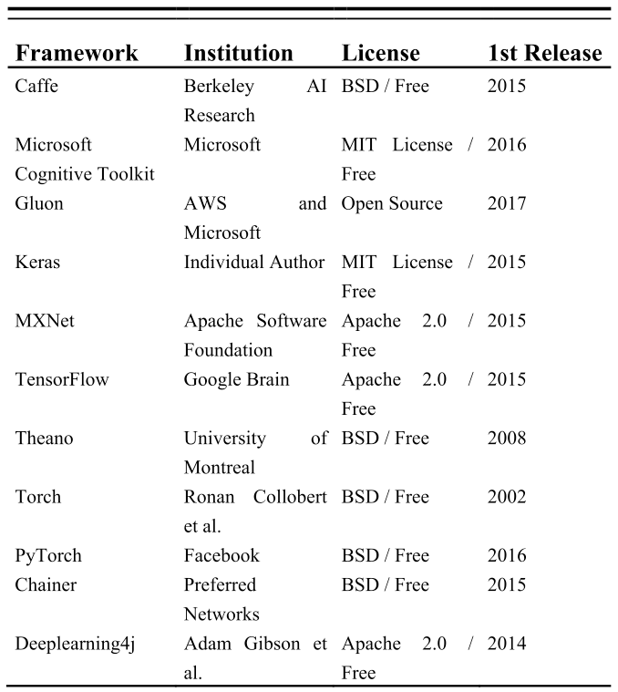
Among these deep learning libraries, TensorFlow currently looks more popular.

Reference:

1. Ajay Shrestha, Ausif Mahmood, Review of Deep Learning Algorithms and Architectures.
2. Deep Learning, Ian Goodfellow, Yoshua Bengio, Aaron Courville.
3. Francois Chollet, Deep Learning with Python.