Review of Deep Learning Algorithms and Architectures III: Autoencoder

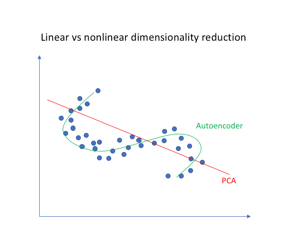
Autoencoders are generalizations of PCA. A PCA transforms multi-dimensional data into a linear representation, whereas, autoencoders go further and produce nonlinear representation.

1. Introduction

Autoencoders use encoder and decoder blocks of non-linear hidden layers to generalize PCA to perform dimensionality reduction and eventual reconstruction of original data.It uses greedy layer by layer unsupervised pretraining and fin-tuning with backpropagation.

Despite using backpropagation, which is mostly used in supervised training, autoencoders are considered unsupervised DNN because they regenerate the input $x^{(i)}$ itself instead of a different set of target values $y^{(i)}$, i.e., $y^{(i)} = x^{(i)}$. Hinton et al. were able to achieve a near perfect reconstruction of 784-pixel images using autoencoder, proving that it is far better than PCA.

2. Mathematical Principles

An antoencoder is defined by the following components:

• Two sets: the space of decoded messages $\mathcal{X}$; the space of encoded messages $\mathcal{Z}$. Almost always, both $\mathcal{X}$ and $\mathcal{Z}$ are Euclidean spaces, that is, $\mathcal{X} = \R_{m}$, $\mathcal{Z} = \R_{n}$ for some $m, n$.

• Two parametrized families of functions: the encoder family $E_{\phi}: \mathcal{X} \rightarrow \mathcal{Z}$, parametrized by $\phi$; the decoder family $D_{\theta}: \mathcal{Z} \rightarrow \mathcal{X}$, parametrized by $\theta$.

For any $x \in \mathcal{X}$, we usually write $\hat{x} = D_{\theta}(z)$, and refer to it as the decoded message.

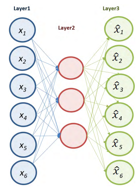
Usually, both the encoder and the decoder are defined are multilayer perceptrons. For example, a one-layer-MLP encoder $E_{\phi}$ is:

$$E_{\phi}(x) = \phi(Wx + b)$$

where $\sigma$ is an element-wise activation function such a sigmoid function or a rectified linear unit, $W$ is a matrix called "weight", and $b$ is a vector called "bias".

The figure below illustrates a simplified representation of how autoencoders can reduce the dimension of the input data and learn to recreate it in the output layer.

3. Training an Autoencoder

An autoencoder is simply a tuple of two functions. To judge its quality, we need a task. A task is defined by a reference probability distribution $\mu_{ref}$ over $\mathcal{X}$, and a "reconstruction quality" function $d: \mathcal{X} \times \mathcal{X} \rightarrow [0, \infty]$, such that $d(x, \hat{x})$ measures how much such $\hat{x}$ differs from $x$. The loss function for the autoencoder can be defined as

$$L(\theta, \phi) := \mathbb{E}_ {x \sim \mu_{ref}}[d(x, D_{\theta}(E_{\phi}(x)))]$$

The optimal autoencoder for the given task $(\mu_{ref}, d)$ is then $\argmin_{\theta, \phi} L(\theta, \phi)$. In most situations, the reference distribution is just the empirical distribution given by a dataset ${x_{1}, ... , x_{N}} \subset \mathcal{X}$, so that

$$\mu_{ref} = \frac{1}{N} \sum_{i=1}^{N} \delta_{x_{i}}$$

and the quality function is just L2 loss: $d(x, \hat{x}) = \parallel x - \hat{x} \parallel_{2}^{2}$.

4. Variations

4.1 Regularized Autoencoders.

The ideal autoencoder model balances the following:

• Sensitive to the inputs enough to accurately build a reconstruction.

• Insensitive enough to the inputs that the model doesn't simply memorize or overfit the training data.

This goal is usually achieved by adding a regularizer to the loss function as a punishment for wildly changed parameters.

$$\mathcal{L}(x, \hat{x}) + \text{regularizer}$$

4.1.1 Sparse Autoencoder (SAE)

Sparse autoencoders are variants of autoencoders, such that the codes $D_{\phi}(x)$ for messages tend to be sparse codes, that is, $D_{\phi}(x)$ is close to zero in most entries. Sparse autoencoders may include more (rather than fewer) hidden units than inputs, but onnly a small number of the hidden units are allowed to be active at the same time.

There are two main ways to enforce sparity. One way is to simple clamp all but the highest-$k$ activation of the latent code to zero. This is the $k$-sparse autoencoder.

The $k$-sparse autoencoder inserts the following "$k$-sparse function" in the latent layer of a standard autoencoder:

$$f_{k}(x_{1}, ... , x_{n}) = (x_{1}b_{1}, ... , x_{n}b_{n})$$

where $b_{i} = 1$ if $| x_{i} |$ ranks in the top $k$, and 0 otherwise.

The other way is a relaxed version of the $k$-sparse autoencoder. Instead of forcing sparsity, we add a sparsity regularization loss, then optimize for

$$\min_{\theta, \phi} L(\theta, \phi) + \lambda L_{sparsity}(\theta, \phi)$$

where $\lambda > 0$ measures how much sparsity we want to enforce.

Assume that the autoencoder architecture have $K$ layers. To define a sparsity regularization loss, we need a "desired" sparsity $\hat{\rho}_ {k}$ for each layer, a weigh $w_{k}$ for how much to enforce each sparsity, and a function $s : [0, 1] \times [0, 1] \rightarrow [0, \infty]$ to measure how much two sparsities differ.

For each input $x$, let the actual sparsity of activation in each layer $k$ be

$$\rho_{k}(x) = \frac{1}{n}\sum_{i=1}^{n} a_{k,i}(x)$$

where $a_{k,i}(x)$ is the activation in the $i$-th neuron of the $k$-th layer upon input $x$.

The sparsity loss unpon input $x$ for one layer is $s(\hat{\rho}_ {k}, \rho_{k}(x))$, and the sparsity regularization loss for the entire autoencoder is the expected weighted sum of sparsity losses:

$$L_{sparsity}(\theta, \phi) = \mathbb{E}_ {x\sim \mu_{X}} [ \sum_{k \ in 1: K} w_{k}]s(\hat{\rho}_ {k}, \rho_{k}(x))$$

Typically, the function $s$ can be one of the following ones:

1. Kullback-Leibler (KL) divergence:

$$s(\hat{\rho}_ {k}, \rho_{k}(x)) = KL(\rho \parallel \hat{\rho})$$

2. L1 Loss:

$$s(\hat{\rho}_ {k}, \rho_{k}(x)) = |\rho - \hat{\rho}|$$

3. L2 Loss

$$s(\hat{\rho}_ {k}, \rho_{k}(x)) = |\rho - \hat{\rho}|^{2}$$

Alternatively, the sparsity regularization loss may be defined without reference to any "desired sparsity", but simply force as much sparsity as possible. In this case, one can sparsity regularization loss as

$$L_{sparsity} (\theta, \phi) = \mathbb{E}_ {x \sim \mu_{X}}[\sum_{k \in 1:K} w_{k} \parallel h_{k}\parallel]$$

where $h_{k}$ is the activation vector in the $k$-th layer of the autoencoder. The norm $\parallel \cdot \parallel$ is usually the L1 norm (giving the L1 sparse autoencoder) or the L2 norm (giving the L2 sparse autoencoder).

4.1.2 Denoising Autoencoder (DAE)

Denoising autoencoders (DAE) try to achieve a good representation by changing the reconstruction criterionn.

A DAE is defined by adding a noise process to the standard autoencoder. A noise process is definned by a probability distribution $\mu_{T}$ over functions $T : \mathcal{X} \rightarrow \mathcal{X}$. That is, the function $T$ takes a message $x\in \mathcal{X}$, and corrupts it to a noisy version $T(x)$. The function $T$ is selected randomly, with a probability distribution $\mu_{T}$.

Given a task $(\mu_{ref}, d)$, the problem of training a DAE is the optimization problem:

$$\min_{\theta, \phi} = \mathbb_{x \sim \mu_{X}, T \sim \mu_{T}}[d(x, (D_{\theta} \circ E_{\phi} \circ T)(x))]$$

That is, the optimal DAE should take any noisy message and attempt to recover the original message without noise, thus the name "denoising". Usually, the noise process $T$ is applied only during training and testing, not during downstream use.

The use of DAE depends on two assumptions:

• There exist representations to the messages that are relatively stable and robust to the type of noise we are likely to encounter;

• The sard representations capture structures in the input distribution that are useful for our purposes.

Example noise processes include:

• Additive isotropic Gaussian noise
• Masking noise (a fraction of the input is randomly chosen and set to 0)
• Salt-and-pepper noise (a fraction of the input is randomly chosen and randomly set to its minimum or maximun value).

4.1.3 Conntractive Autoencoder (CAE)

A contractive autoencoder adds the contractive regularization loss to the standard autoencoder loss:

$$\min_ {\theta, \phi} + \lambda L_{contractive} (\theta, \phi)$$

where $\lambda > 0$ measures how much contractiveness we want to enforce. The contractive regularization loss itself is defined as the expected Frobenius norm of the Jacobian matrix of the encoder activations with respect to the inputs:

$$L_{contractive} (\theta, \phi) = \mathbb{E}_ {x \sim \mu_{ref}} \parallel \nabla_{x}E_{\phi}(x) \parallel_{F}^{2}$$

To understand what $L_{contractive}$ measures, note the fact

$$\parallel E_{\phi}(x+\delta x) - E_{\phi} (x) \parallel_{2} \leq \parallel \nabla_{x}E_{\phi}(x) \parallel_{F} \parallel \delta x \parallel_{2}$$

for any message $x \in \mathcal{X}$, and small variation $\delta x$ in it. Thus, if $\parallel \nabla_{x}E_{\phi}(x) \parallel_{F}^{2}$ is small, it means that a small neighborhood of the message maps to a small neighborhood of its code. This is a desired property, as it means small variation in the message leads to small, perhaps even zero, variation in its code, like how two pictures may look the same even if they are not exactly the same.

The DAE can be understood as an infinitesimal limit of CAE: in the limit of small Gaussian input noise, DAEs make the reconstruction function resist small but finite-size input perturbations, while CAEs make the extracted features resist infinitesimal input persturbations.

4.2 Concrete Autoencoder

The concreteb autoencoder is designed for discrete feature selection. A concrete autoencoder forces the latent space to consist only of a user-specified number of features. The concrete autoencoder uses a continuous relaxation of the categorical distribution to allow gradients to pass through the feature seletor layer, which makes it possible to use standard backpropagation to learn an optimal subset of input features that minimize reconstruction loss.

4.3 Variational Autoencoder (VAE)

Variational autoencoders (VAEs) belong to the families of variational Bayesian methods. Despite the architectural sinilarities with basic autoencoders, VAEs aer architecture. with different goals and with a completely different mathematical formulation. The latent space is in this case composed by a mixture of distributions instead of a fixed vector.

Given an input dataset $x$ characterized by an unknown probability function $P(x)$ and a multivariate encoding vector $z$, the objective is to model the data as a distribution $p_{\theta}(x)$, with $\theta$ defined as the set of the network parameters so that $p_{\theta}(x) = \int_{z} p_{\theta}(x, z)dz$.