
Review of Deep Learning Algorithms and Architectures V: RNN and LSTM
1. Brief Introduction to Recurrent Neural Networks
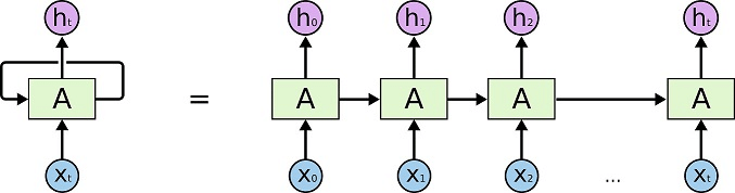
Recurrent neural networks or RNNs (Rumelhart et al., 1986) are a family of neural networks for processing sequential data. Just like the other neural networks that we've seen before, recurrent neural networks have weights, biases, layers and activation functions. The big difference is that RNNs also have feedback loops, which makes it possible to use sequential input values (as illustrated below), like stock market prices collected over time, to make predictions.
Here we need to point out the advantage of this 'unfold' process -- the weights and biases are shared across every input, in other words, parameters sharing. That makes it possible to extend and apply the model to examples of different forms (different lengths, for example) and generalize across them.
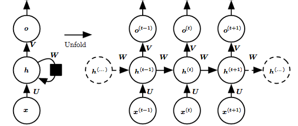
So, no matter how many times we unroll a recurrent neural network, we never increase the number of weights and biases that we have to train.
Despite the advantage, RNNs still have some problems. One big problem is that the more we unroll a recurrent neural network, the harder it is to train due to the vanishing/exploding gradient issue. For example, if one of the weights is $2$ and the RNN is unrolled by 50 times, then the final weight will rise to $2^{50}$, which is really huge and it will cause an exploding gradient problem. That would make it hard to take small steps to find the optimal weights and biases.
One way to prevent the exploding gradient problem would be to limit the weight $w$ to values less than 1. However, this results in the vanishing gradient problem.
2. Leaky Units and Other Strategies for Multiple Time Scales
One way to deal with long-term dependencies, or vanishing/exploding gradient problem is to design a model that operates at fine-grained time scales and can handle small details, while other parts operate at coarse time scales and transfer information from the distant past to the present more efficiently.
Various strategies for building both fine and coarse time scales are possible.
2.1 Adding Skip Connections through Time
One way to obtain coarse time scales is to add direct connections from variables in the distant past to variables in the present. In an ordinary recurrent network, a recurrent connection goes from a unite at time $t$ to a unit at $t+1$. It is possible to construct recurrent connection with longer delays.
Lin et al. (1996) introduced recurrent connection with a time delay of $d$ to mitigate this problem. Assume a recurrent neural network is specialized for processing a sequence of values $\mathbf{x}^{(1)}, \ldots, \mathbf{x}^{(\tau)}$, the gradient now diminish exponentially as a function of $\frac{\tau}{d}$ rather than $\tau$.
Since there are both delayed and single step connections, gradients may still explode exponentially in $\tau$. This allows the learning algorithm to capture longer dependencies, although not all long-term dependencies may be represented well in this way.
2.2 Leaky Units and a Spectrum of Different Time Scales
Another way to obtain paths on which the product of derivatives is close to one is to have units with linear self-connections and a weight near one on these connections.
When we accumulate a running average $\mu ^{t}$ of some value $v ^{t}$ by applying the update $\mu ^{t} \leftarrow \alpha \mu ^{(t-1)} + (1 - \alpha) v ^{(t)}$, the $\alpha$ parameters is an example of a linear self-connection from $\mu ^{(t-1)}$ to $\mu ^{t}$. When $\alpha$ is near one, the running average remembers about the past for a long time, and when $\alpha$ is near zero, information about the past is rapidly discarded. Hidden units with linear self-coonections can behave similarly to such running average. Such hidden units are called leaky units.
There are two basic strategies for setting the time constants used by leaky units. One strategy is to manually fix them to values that remain constant, for example, by samplinng their values from some distribution once at initialization time. Another strategy is to make the time constants free parameters and learn them. Having such leaky units at different time scles appears to help with long-term dependencies.
2.3 Removing Connections
Another approach to handling long-term dependencies is the idea of organizing the state of the RNN at multiple time scales with information flowing more easily through long distances at the slower time scales.
This idea differs from the skip connections through time discussed earlier because it involves actively removing length-one connections and replacing them with longer connections. Units modified in such a way are forced to operate on a long time scale. Skip connections through time add edges. Units receiving such new connections may learn to operate on a long time scale but may also choose to focus on their other, short-term connections.
There are different ways in which a group of recurrent units can be forced to operate at different time scales. One option is to make the recurrent units leaky, but to have different groups of units associated with different fixed time scales. Another option is to have explicit and discrete updates taking place at different times, with a different frequency for different groups of units.
3. Long Short-Term Memory (LSTM)
We've briefly intorduced vanilla Recurrent Neural Networks (RNNs), and showed how we can use a feedback loop to unroll a network that works well with different amounts of sequential data. Also, we mentioned the vanishing/exploding gradient issues may appear in the RNN training process and some strategies to relief this issue.
Now, we're going to talk about Long Short-Term Memory (LSTM), which is a type of RNN that is designed to avoid the exploding/vanishing gradient problem.
The main idea behind how LSTM works is that instead of using the same feedback loop connection for events that happens long ago and events that just happened yesterday to make a prediction about tomorrow. Long Short-Term Memory uses two separate paths to make predictions about tomorrow. One path for Long-Term Memories and one is for Short-Term Merories.
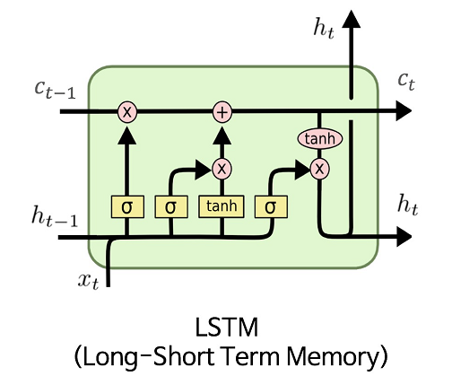
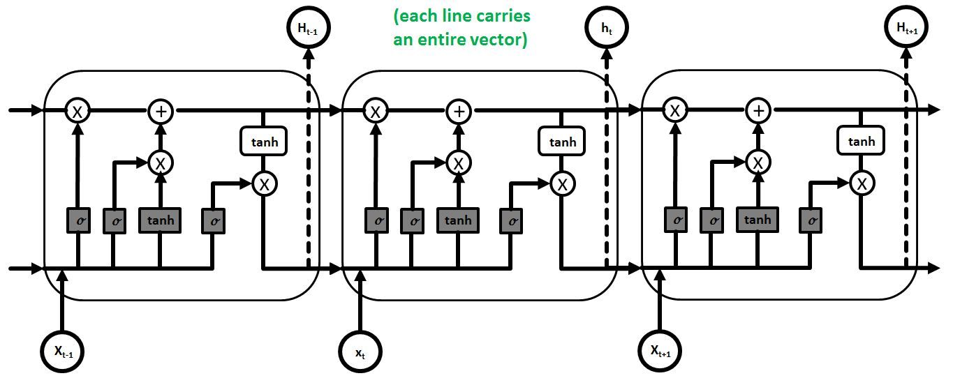
Compared to a basic, vanilla recurrent neural network, which unfolds from a relatively simple unit, Long Short-Term Memory is based on a much more complicated unit illustrated below.
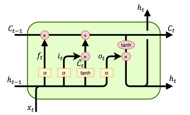
In this figure, $C$, $x$, $h$ represent cell (represents the Long-Term Memory), input and output (represents Short-Term Memory) values. Subscript $t$ denotes the time step value, i.e., $t-1$ is from previous LSTM block (or from time $t-1$) and $t$ denotes current block values. The symbol $\sigma$ is the sigmoid function and $\tanh$ is the hyperbolic tangent function. Operator $+$ is the element-wise summation and operator $\otimes$ is the element-wise multiplication. The computations of the gates are described in the equations below.
$f_{t} = \sigma (W_{f}\cdot[h_{t-1}, x_{t}] + b_{f})$
$i_{t} = \sigma (W_{i}\cdot[h_{t-1}, x_{t}] + b_{i})$
$o_{t} = \sigma (W_{o}\cdot[h_{t-1}, x_{t}] + b_{o})$
$\tilde{C}_ {t} = \tanh(W_{C}\cdot[h_{t-1}, x_{t}] + b_{C})$
$C_{t} = f_{t} \otimes C_{t-1} + i_{t} \otimes \tilde{C}_ {t}$
$h_{t} = o_{t} \otimes \tanh (C_{t})$
where $f$, $i$, $o$ are the forget, input and output gate vectors respectively. Their functions can be briefly explained as follows:
- Forget gate determines what percentage of the Long-Term Memory is remembered.
- Input gate combines the Short-Term Memory and the input to create a Potential Long-Term Memory $\tilde{C}$ and determines what percentage of that Potential Memory to add to Long-Term Memory.
- Output gate updates the Short-Term Memory and produces the output from this the entire LSTM unit.
Please note that although the Long-Term Memory can be modified by the multiplaction and addition, there are no weights and biases that can modify it directly. This lack of weights allows the Long-Term Memories to flow through a series of unrolled units without causing the gradient to explode or vanish.
Now, we unfold the loop and obtain a of LSTM unit chain.
The LSTM has been found extremely successful in many applications, such as unconstrained handwriting recognition, speech recognition, handwriting generation, image captioning, and parsing.
Reference:
- Deep Learning, Ian Goodfellow, Yoshua Bengio, and Aaron Courville.
- Review of Deep Learning Algorithms and Architectures, Ajay Shrestha and Ausif Mathmood.
In addition to the reference mentioned above, I highly recommend a video on Youtube, Long Short-Term Memory, Clearly Explained produced by StatQuest with Josh Starmer. Josh has a talent for explaining mathematics, statistics, and machine learning in plain language. I learned a lot from his channel.