Sparse Quasi-Markowitz Portfolio (SQMP)

• According to a 2020 report, over a 15-year period, nearly 90% of actively managed investment funds failed to beat the market. This may not surprise you. But back in 1976, when Bogle created the First Index Investment Trust as the first index mutual fund available to the general public, passive investment sounded crazy at that time.

• Index funds are essentially portfolios of stocks that are managed by a professional financial firm, which tries to copy the performance of the index. For example, a particular stock makes up 1% of the index, then the firm managing the index fund will seek to mimic that same composition by making 1% of its portfolio consist of that stock.

• In general, index funds have lower expense ratios. Transaction cost is the main component of fund expense. The weights of the component stocks in the index vary now and then, so the portfolio tracking the index needs to be adjusted accordingly. If the number of component stocks is large, then the reweighting cost is nonnegligible.

• Now we introduce a method to construct a sparse quasi-Markowitz portfolio that may beat the index funds and reduce transaction cost at the same time.

Modern Portfolio Theory (MPT)

• Modern Portfolio Theory (MPT), or mean-variance analysis, is a mathematical framework for assembling a portfolio of assets such that the expected return is maximized for a given level of risk. This optimization problem can be solved by quadratic programming, on the condition that the expected return and covariance matrix of asset returns can be estimated precisely.

• Unfortunately, those parameters are not observed in practice, in this case, the sample mean and sample covariance matrix are used as proxies, and the resulting "plug-in" portfolio, which has been studied by ample researchers, whose performance is pretty unacceptable.

An Unconstrained Regression Representation

• Suppose that we have a pool of \(N\) risky assets. Denote their (random excess) returns by \(\boldsymbol{r}=(r_{1}, r_{2}, \ldots, r_{N})'\). Let \(\boldsymbol{\mu}\) and \(\boldsymbol{\Sigma}\) be the mean vector and covariance matrix of \(\boldsymbol{r}\), respectively, and let \(\boldsymbol{w}\) be a vector of portfolio weights on the assets. For a given risk constraint \(\sigma\), the mean-variance portfolio problem is

\[\underset{\boldsymbol{w}}{\arg \max } E\left(\boldsymbol{w}^{\prime} \boldsymbol{r}\right)=\boldsymbol{w}^{\prime} \boldsymbol{\mu} \quad \text { subject to } \quad \operatorname{Var}\left(\boldsymbol{w}^{\prime} \boldsymbol{r}\right)=\boldsymbol{w}^{\prime} \boldsymbol{\Sigma} \boldsymbol{w} \leq \sigma^{2} \]

• If we denote \(\theta = \boldsymbol{\mu}'\boldsymbol{\Sigma}^ {-1}\boldsymbol{\mu}\) as the square of the maximum Sharpe ratio of the optimal portfolio, then the optimization problem can be represented in its dual form with a return constraint:

\[\underset{\boldsymbol{w}}{\arg \min } \boldsymbol{w}^{\prime} \boldsymbol{\Sigma} \boldsymbol{w} \quad \text { subject to } \quad \boldsymbol{w}^{\prime} \boldsymbol{\mu} \geq r^{*}:=\sigma \sqrt{\theta} \]

• The optimal portfolio, \(\boldsymbol{w}*\), admits the following explicit expression:

\[\boldsymbol{w}^{*}=\frac{\sigma}{\sqrt{\theta}} \boldsymbol{\Sigma}^{-1} \boldsymbol{\mu}\]

• Encumbered by the difficulty of the high-dimensional covariance matrix, the portfolio has given above usually has poor performance. Now we introduce an equivalent and unconstrained regression of mean-variance optimization.

• Construct the unconstrained regression:

\[\underset{\boldsymbol{w}}{\arg \min } E\left(r_{c}-\boldsymbol{w}^{\prime} \boldsymbol{r}\right)^{2}, \quad \text { where } \quad r_{c}:=\frac{1+\theta}{\theta} r^{*} \equiv \sigma \frac{1+\theta}{\sqrt{\theta}}\]

is equivalent to the mean-variance optimizations mentioned above.

• Estimate the optimal portfolio by replacing \(\underset{\boldsymbol{w}}{\arg \min } E\left(r_{c}-\boldsymbol{w}^{\prime} \boldsymbol{r}\right)^{2}\) with its sample version

\[\underset{\boldsymbol{w}}{\arg \min } \frac{1}{T} \sum_{t=1}^{T}\left(r_{c}-\boldsymbol{w}^{\prime} \boldsymbol{R}_{t}\right)^{2}\]

where \(\boldsymbol{R}_ {t} = (R_{t1}, \ldots, R_{tN})', t=1, \ldots, T\) are \(T\) i.i.d. copies of the return vector \(\boldsymbol{r}\).

• Since consistently estimating the coefficients in high-dimensional regression is, in general, impossible, some type of sparsity is required to make it possible.

• The sparse regression corresponding to the optimization is:

\[\boldsymbol{w}\left(r_{c}\right):=\underset{\boldsymbol{w}}{\arg \min } \frac{1}{T} \sum_{t=1}^{T}\left(r_{c}-\boldsymbol{w}^{\prime} \boldsymbol{R}_ {t}\right)^{2} \quad \text { subject to } \quad ||\boldsymbol{w}||_ {1} \leq \lambda\]

• A feasible LASSO-type estimator \(\widehat{\boldsymbol{w}^{*}}=\left(\widehat{w_{1}^{*}}, \ldots, \widehat{w_{N}^{*}}\right)^{\prime}\) can be constructed as follows:

\[\widehat{\boldsymbol{w}^{*}}= \underset{\boldsymbol{w}}{\arg \min } \frac{1}{T} \sum_{t=1}^{T}\left(\widehat{r}_ {c}-\boldsymbol{w}^{\prime} \boldsymbol{R}_ {t}\right)^{2} \quad \text { subject to } \quad ||\boldsymbol{w}||_{1} \leq \lambda\]

• How different \(\lambda\) values effect the portfolios' performance?

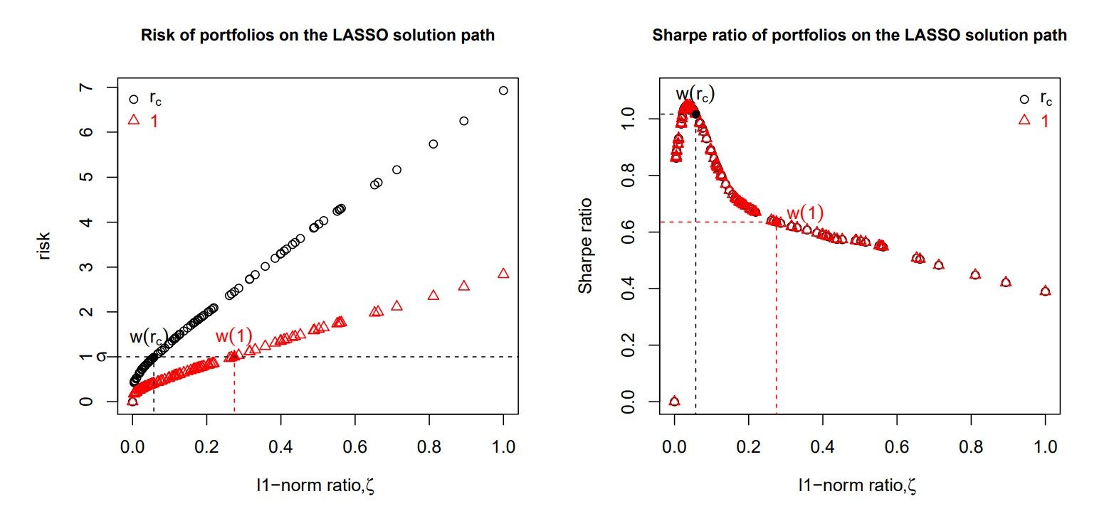
• In the figure below, two LASSO solution paths are presented, one with response \(r_{c}\) (setting \(\sigma=1\)) and the other with response 1. The x-axix represents the ratio of the \(l_{1}\)-norm of a solution, \(\boldsymbol{w}\), on the solution path relative to that of the OLS solution:

\[\zeta=\frac{||\boldsymbol{w}||_ {1}}{||\boldsymbol{w}_ {ols}||_{1}}\]

• We have the following observation:

  1. For each solution path, the risk increases with respect to the \(l_{1}\)-norm ratio \(\zeta\).
  2. Regarding the Sharp ratio comparison, we see that the Sharpe ratio paths coincide. The portfolio with the correct response \(r_{c}\) achieves almost the highest Sharpe ratio on the path.

• Now two important questions to answer:

  1. How to determine the right value for \(r_{c}\)?
  2. How to determine the right value for \(\lambda\)?

• We don't want to get trapped in the technical details. Here we just give you a brief hint for these two questions:

  1. Estimate \(\theta\) via factor model (Fama factor model, for example), then you obtain an estimate of \(r_{c}\) by \(\widehat{r_{c}}:=\sigma \frac{1+\widehat{\theta}}{\sqrt{\hat{\theta}}}\).
  2. Find the right value of \(\lambda\) by k-fold cross-validation.

• By now we show the whole construction process of the Sparse Quasi-Markowitz Portfolio (SQMP) to you. According to some researches, SQMP has a better performance compared to the traditional Markowitz Portfolio. What makes it more attractive is that usually, it can also beat the index-tracking portfolio with a lower transaction fee.