Oct 11, 2021 4 min read

What is Latent Semantic Analysis (LSA)

Short Answer

Latent semantic analysis (LSA) is a natural language processing technique for analyzing documents and terms contained within them.
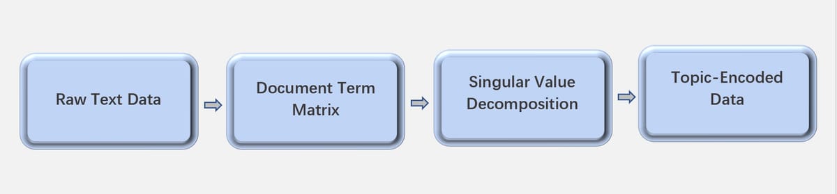
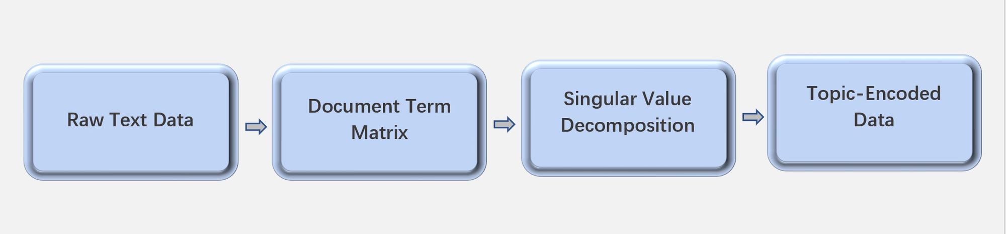
Generally speaking, we can procedure LSA in 4 steps:
1. Collect, clean, and prepare text data for further analysis.
2. Build document term matrix from the cleaned text documents.
3. Perform singular value decomposition on the document term matrix.
4. Look at the topic encoded data that came out of the singular value decomposition.

lsa1-1

Long Answer

Although LSA seems easy in our short answer, there are still many questions about the process. How to clean the text data? How to transform words into feature vectors? How to perform singular value decomposition? And why does that matter when we try to analyze the sentiment of the text? Now we will give a more detailed explanation for the four steps we mentioned above.

1. Collect, Clean, and Prepare Text Data

In most cases, the raw text is stored in a file, for instance, a CSV file. We need to read the file and have a look at the dataset.

df = pd.read_csv('movie_data.csv', encoding='utf-8')

Sometimes there are several nonsense symbols, such as \ : % & $, in the text. Python has a package named re, which can help you to get rid of these nonsense symbols by using regular expressions.

2. Build Document Term Matrix

A document term matrix is generally a high-dimensional sparse matrix. The columns represent the unique words contained in the collection of documents. The rows represent the documents or paragraphs to be analyzed.
The simplest method to transform words into feature vectors is to use the bag-of-words model. To construct a bag-of-words model based on the word counts in the respective documents, we can use the CountVectorizer class in the scikit-learn package.

from sklearn.feature_extraction.text import CountVectorizer
count = CountVectorizer()
bag = count.fit_transform(docs)

Through a toy example, you could figure out what does the matrix look like.

	the	book	is	good	I	like	it	books	a	table
The book is good	1	1	1	1	0	0	0	0	0	0
I like it	0	0	0	0	1	1	1	0	0	0
I like good books	0	0	0	1	1	1	0	1	0	0
Book a table	0	1	0	0	0	0	0	0	1	1

By calling the fit_transform method on CountVectorizer, we transform four pieces of text into sparse feature vectors.

Before we striding to the next step, let's look at the matrix for a while. You will notice, some columns are not very informative, for example, the article words, 'a', 'an', and 'the', and some other words like, 'has', 'are', and so on. In the language natural processing world, we call these words stop-words.
We may also encounter some words that occur across multiple documents, for example, 'I', 'do', 'take', etc. If we use word count directly, these frequently occurring works typically have a big counting number, but that doesn't deliver too much useful or discriminatory information to us. Here, we introduce a helpful technique called the term frequency-inverse document frequency (tf-idf), which can be used to down weight the frequently occurring words in the feature vectors.
The tf-idf can be defined as the product of the term frequency (tf) and the inverse document frequency (idf) as follows:

\[tf-idf(t, d)= tf(t, d) \times idf(t, d) \]

where $tf(t, d)$ is the term frequency -- the number of times a term, $t$, occurs in a document, $d$.

The inverse document frequency, $idf(t, d)$, which indicate the rarity of the word, can be calculated as follows:

\[idf(t, d) = log \frac{1+n_{d}}{1+df(d, t)}\]

Here, $n_{d}$ is the total number of documents, and $df(d, t)$ is the number of documents, $d$, that contain the term $t$.

You can see, if all documents we considered containing term $t$, then $idf(t, d)$ will be 0, that makes the value of $td-idf(t, d)$ 0 too.
The scikit-learn library implements yet another transformer, the TfidTransformer class, which takes the raw term frequencies from the CountVectorizer class as input and transforms them into tf-idfs. Amazingly, the stop-words can be removed at the same time.

from sklearn.feature_extraction.text import TfidfVectorizer
tfidf = TfidfVectorizer(min_df=1, stop_words='english')
doc_matrix = tfidf.fit_transform(bag)

3. Singular Value Decomposition

Let $\boldsymbol{M}$ denotes the $m \times n$ document term matrix, which has sigular value decomposition (SVD):

\[\boldsymbol{M} = \boldsymbol{U\Sigma V^{T}}\]

where $\boldsymbol{U}$ is an $m \times m$ orthogonal matrix, $\boldsymbol{V}^{T}$ is an $n \times n$ orthogonal matrix, and the diagonal entries of $\boldsymbol{\Sigma}$ are known as the sigular values of $\boldsymbol{M}$.

It is always possible to choose the decomposition so that the singular values are in descending order.

For most cases, we don't need the full singular decomposition. Since the singular values approaching 0 may not provide much useful information for us, we can just ignore them and truncate the singular decomposition, which can be achieved using the TrancatedSVD method in scikitlearn.
Python codes for SVD

from sklearn.decomposition import TruncatedSVD
svd = TruncatedSVD(n_components=d)
lsa = svd.fit_transform(doc_matrix)

Note that by executing the codes above, only the $d$ largest diagonal entries in the singular value matrix are kept. That reduces the feature space to $d$ dimension, which is usually much smaller comparing to the dimension of the original feature space.
We get the rank $d$ approximation to $\boldsymbol{M}$, which makes us can treat the term and document vectors as a 'semantic space'. We write this approximation as

\[\boldsymbol{M}_{d} = \boldsymbol{U}_{d}\boldsymbol{\Sigma} _{d}\boldsymbol{V}_{d}^{T}\]

4. Topic-Encoded Data

We can access topic-encoded data via the codes below:

import pandas as pd
topic_endode_df = pd.DataFrame(lsa, columns = ['topic_1', 'topic_2',...,'topic_d'])

The document term matrix in $d$-dim semantic space is $\boldsymbol{U}_ {d}\boldsymbol{\Sigma}_ {d}\boldsymbol{V}_ {d}^{T}$. Note that $\boldsymbol{U}_ {d}$ is an $m \times d$ matrix, $\boldsymbol{\Sigma}_ {d}$ is a $d \times d$ matrix, and $\boldsymbol{V}_ {d}^ {T}$ is a $d \times n$. Although $\boldsymbol{U}_ {d}\boldsymbol{\Sigma}_ {d}\boldsymbol{V}_ {d}^{T}$ is still an $m \times n$ matrix, the elements in it changes a lot. The new matrix represents new information delivered by those original texts in the semantic space. Additionallty, the similarity between word and word or text and text also changed in this space.