High Dimensional Covariance Matrix Estimation


Covariance matrix estimation is fundamental for almost all areas of multivariate analysis and many other applied problems. For instance, according to Markowitz's portfolio theory, the eigenvectors of the return covariance matrix determine the portfolio allocation.
Intuitive thought is to take the sample covariance matrix as the estimation of the general covariance matrix. However, sample covariance usually has a pretty poor performance when the dimension gets large.
Given the importance of covariance matrix estimation, several approaches were proposed in the literature to construct good covariance matrix estimators. Among them, two main directions were taken:
- To remedy the sample covariance matrix and construct a better one by using approaches such as shrinkage and the eigen-method, etc.
- To reduce dimensionality by imposing some structure on the data. Many structures, such as sparsity, compound symmetry, and the autoregressive model, are widely used.
Empirical researches have confirmed that usually, these improved estimators have better performance compared to the sample covariance matrix. It is worth noting that when we encounter a specific problem, we might have more information about the variables. In that case, by utilizing the new information, the estimator can be improved even further.
For example, factor models are widely used in past decades to estimate the return of the individual stock. By the Arbitrage Pricing Theroy, the excessive return of any asset \(Y_{i}\) over the risk-free interest rate satisfied
\[Y_{i}=b_{i 1} f_{1}+\cdots+b_{i K} f_{K}+\varepsilon_{i}, \quad i=1, \cdots, p \]
where \(f_{1}, \cdots, f_{K}\) are the excessive returns of \(K\) factors, \(b_{i j}, i=1, \cdots, p, j=1, \cdots, K\) are unknown factor loadings, and \(\varepsilon_{1}, \cdots, \varepsilon_{p}\) are \(p\) idiosyncratic errors uncorrelated given \(f_{1}, \cdots, f_{K}\).
Perhaps the most famous special case of the factor model is the Capital Asset Pricing Model (CAPM), which will be used in our estimator. We don't want to rush to the final results. For the sake of wider application, a general covariance matrix estimator based on the factor model should be given first.
Let \(n\) denotes the smaple size, \(p\) denotes the dimensionality, and \(f_{1}, \cdots, f_{K}\) denotes the \(K\) observable factors. For simplarity of notation, we rewrite factor model in matrix form
\[\mathbf{y}=\mathbf{B}_{n} \mathbf{f}+\varepsilon\]
where \(\mathbf{y}=\left(Y_{1}, \cdots, Y_{p}\right)^{\prime}, \mathbf{B}_ {n}=\left(\mathbf{b}{1}, \cdots, \mathbf{b}{p}\right)^{\prime}\) with \(\mathbf{b}_ {i}=\left(b_{n, i 1}, \cdots, b_{n, i K}\right)^{\prime}, i=1, \cdots, p,\) \(\mathbf{f}=\left(f_{1}, \cdots, f_{K}\right)^{\prime}, \) and \( \mathbf{\varepsilon}=\left(\varepsilon_{1}, \cdots, \varepsilon_{p}\right)^{\prime}\). We further assume that \(E(\mathbf{\varepsilon} \mid \mathbf{f})=\mathbf{0}\) and \( cov (\mathbf{\varepsilon} \mid \mathbf{f})=\boldsymbol{\Sigma}_ {n, 0}\) is diagonal.
For convenience, we introduce more notations below.
\[\mathbf{\Sigma}_ {n} = \operatorname{cov}(\mathbf{y}), \mathbf{X}=\left(\mathbf{f}_{1}, \cdots, \mathbf{f}_{n}\right), \mathbf{Y}=\left(\mathbf{y}_{1}, \cdots, \mathbf{y}_{n}\right), \text{ and } \mathbf{E}=\left(\varepsilon_{1}, \cdots, \varepsilon_{n}\right).\]
Under factor model, we have
\[ \boldsymbol{\Sigma}_{n}= \operatorname{cov} \left(\mathbf{B}_{n} \mathbf{f}\right)+\operatorname{cov}(\boldsymbol{\varepsilon})=\mathbf{B}_{n} \operatorname{cov}(\mathbf{f}) \mathbf{B}_{n}^{\prime}+\boldsymbol{\Sigma}_{n, 0}.\]
Fan (2006) proposed a natural idea for estimating \(\boldsymbol{\Sigma}_ {n}\) is to plug in the least-squares estimators of \(\boldsymbol{B}_ {n}\), \(cov (\boldsymbol{f})\) and \(\boldsymbol{\Sigma}_ {n, 0}\). Therefore, they got a substitution estimator
\[\widehat{\boldsymbol{\Sigma}}_{n}=\widehat{\mathbf{B}}_{n} \widehat{\operatorname{cov}}(\mathbf{f}) \widehat{\mathbf{B}}_{n}^{\prime}+\widehat{\boldsymbol{\Sigma}}_{n, 0}\]
where \(\widehat{\mathbf{B}}_ {n}=\mathbf{Y} \mathbf{X}^{\prime}\left(\mathbf{X X}{\prime}\right){-1}\) is the matrix of estimated regression coefficients, \(\widehat{\operatorname{cov}}(\mathbf{f})=(n-1)^{-1} \mathbf{X X}{\prime}-{n(n-1)}{-1} \mathbf{X} \mathbf{1 1}^{\prime} \mathbf{X}^{\prime}\) is the sample covariance matrix of the factor \(\mathbf{f}\), and
\[\widehat{\boldsymbol{\Sigma}}_{n, 0}=\operatorname{diag}\left(n^{-1} \widehat{\mathbf{E}} \widehat{\mathbf{E}}^{\prime}\right)\]
where \(\widehat{\mathbf{E}}=\mathbf{Y}-\widehat{\mathbf{B}} \mathbf{X}\) is the matrix of residuals.
The author concluded that comparing the sample covariance matrix \( \widehat{\boldsymbol{\Sigma}}_ {\mathrm{sam}}\) the substitution estimator \( \widehat{\boldsymbol{\Sigma}}\) had several advantages:
- \( \widehat{\boldsymbol{\Sigma}}\) is always invertible, even if \( p > n \), while \( \widehat{\boldsymbol{\Sigma}}_ {\mathrm{sam}}\) suffers from the problem of possibly singular when dimensionality \( p\) is close to or larger than sample size \( n\).
- \( \widehat{\boldsymbol{\Sigma}}\) has asymptotic normality, while \( \widehat{\boldsymbol{\Sigma}}_ {\mathrm{sam}}\) may not have asymptotic normality of the same kind.
Recall that the Markowitz portfolio, \(\boldsymbol{w}*\), admits the following explicit expression:
\[\boldsymbol{w}^{*}=\frac{\sigma}{\sqrt{\boldsymbol{\mu}'\boldsymbol{\Sigma}^ {-1}\boldsymbol{\mu}}} \boldsymbol{\Sigma}^{-1} \boldsymbol{\mu}\]
where \(\boldsymbol{\mu}\) and \(\boldsymbol{\Sigma}\) denote the mean vector and covariance matrix of \(\boldsymbol{r}\), respectively, and \(\boldsymbol{w}\) represents a vector of portfolio weights on the assets, given a risk constraint \(\sigma\).
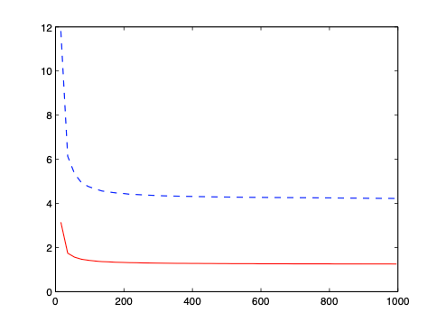
Plugging two estimators into the weight formular respectively, we obtain two optimal portfolios. The figure below shows MSEs of estimated variances of the optimal portfolios based on \( \widehat{\boldsymbol{\Sigma}}\) (solid curve) and \( \widehat{\boldsymbol{\Sigma}}_ {\mathrm{sam}}\) (dashed curve) against \( p\). We can see estimator \( \widehat{\boldsymbol{\Sigma}}\) real performs better.
Although the idea behind this covariance matrix estimation is simple and intuitive. It went unnoticed by the statisticians and practitioners until 2006 when Fan first proposed this estimator and studied it thoroughly. We will see in a future post that we can improve this estimator further with another simple and intuitive idea.