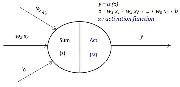
Activation Functions III: Trainable Activation Functions

Introduction

The idea of traninable activation functions is not new in the neural networks research field. In recent years, as training data increases and the cost of computation decreases, the renewed interest in neural networks has led the research to consider again the hypothesis that trainable activation functions could improve the performance of neural networks.

In this blog we describe and analyze the main methods presented in the literature related to the activation functions that can be learned by data. Relying on their main characteristics, trainable activation functions can be divided into two distinct families:

• Parameterized standard activation functions.
• Activation functions based on ensemble methods.

With parameterized standard activation functions we refer to all the functions with a shape very similar to a given fixed-shape function, but tuned by a set of trainable parameters; with ensemble methods we refer to any technique merging different functions.

1. Parameterized Standard Activation Functions

As mentioned above, with the expression "parameterized standard activation functions" we refer to all the functions with a shape very similar to a given fixed-shape function, but having a set of trainable parameters that let this shape to be tuned.

In the remainder of this blog, we will give a brief introduction to these functions. Some of them are plotted in the figure below.

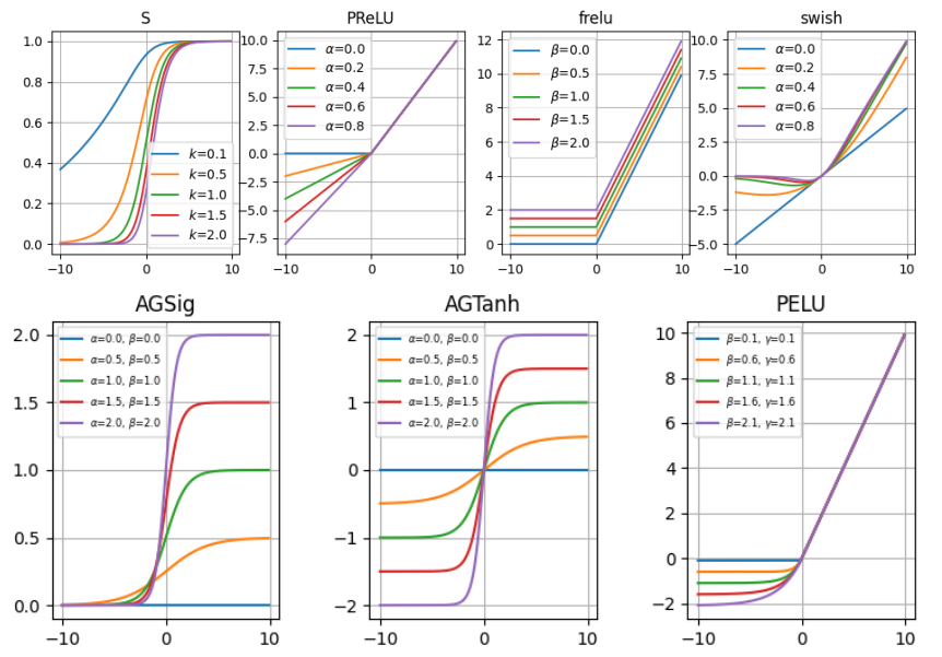
Adjustable Generalized Sigmoid

The first attempt to have a trainable activation function is proposed by Hu and Shao. They add two parameters $\alpha, \beta$ to the classic sigmoid function to adjust the function shape, i.e.:

Both parameters are learned together using a gradient descent approach based on backpropagation algorithm to compute the derivatives of the error function with respect to the network parameters.

Sigmoidal Selector

Singh and Chandra propose the following class of sigmoidal functions, which has a trainable parameter $k$:

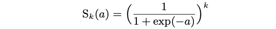
In their paper, the parameter $k$ is learned together with the other network parameters by the gradient descent and back propagation algorithms.

Adjustable Generalized Hyperbolic Tangent

This activation function is proposed by Chen and Change. It generalizes the classic hyperbolic tangent function Tanh by introducing two trainable parameters $\alpha, \beta$:

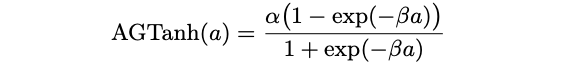
In this function, $\alpha$ adjusts the saturation level, while $\beta$ controls the slope. These two parameters are learned together with th network weights using the classic gradient descent algorithm combined with back-propagation, initializing all the values randomly.

Parametric ReLU

This activation function is introduced by He et al, which partially learns its shape from the training set, in fact, it can modify the negative part using a parameter $\alpha$:

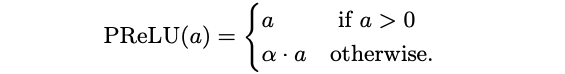
The parameter $\alpha$ is learned jointly with the whole model using classical gradient-based methods with backpropagation without weight decay to avoid pushing $\alpha$ to zero during the training. Empirical experiments show that the magnnitude of $\alpha$ rarely is larger than 1, although no special connstraints on its range are applied.

Parametric ELU

Trottier et al. try to eliminate the need to manually set the $\alpha$ parameter of ELU unit by proposing an alternative version based on two trainable parameters, i.e.:

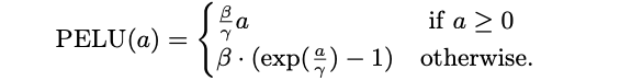
The positive parameters $\beta, \gamma$ control the function shape and are learned together with the other network parameters using some optimization gradient-based method.

Flexible ReLU

Qiu et al. propose the following function:

$$frelu(a) = ReLU(a+ \alpha) + \beta$$

with $\alpha, \beta$ learned by data. This is done to capture the negative information which is lost with the classic ReLU function and to provide the zero-like property. Considering that the value of $a$ is a weighted sum of inputs and bias, the $\alpha$ parameter can be viewed as part of the function input, so the authors reduced the function to

$$frelu(a) = ReLU(a) + \beta.$$

Swish

Ramachandran et al. propose a search technique for activation functions. In a netshell, a set of candidate activation functions is built by combining functions belonging to a predefined set of basis activation functions. For each canndidate activation function, a network which uses generated function is trained on some task to evaluate the performance. Among all the tested functions, the best one results to be:

$$Swish(a) = a\cdot \sigma(\alpha \cdot a)$$

where $\alpha$ is a trainable parameter. It is worth to point out that for $\alpha \rightarrow + \infty$, Swish behaves as ReLU, while, if $\alpha = 1$, it becomes equal to SiLU.

Discussion

In general, the trained acctivation function shape turns out to be very similar to its corresponding non-trainable version, with the result of a poor increase of its expressiveness. For examplem, in the figure above, you can see that the AGSig/AGTanh function results to be the Sigmoid/Tanh function with smoothness and amplitude tuned by the $\alpha$ and $\beta$ parameters. Simalarly, Swish can be viewed as a parameterized SiLU/ReLU variation whose final shape is learned to have a good trade-off between these two functions. In the end, the general function shape remains substantially bounnded to assume the basic function(s) shape on which it has been built.

However, being the most significant part of these functions just a weighted output of the respective weighted input of a fixed activation function, one can notice that it is possible to model each of them by a simple shallow neural subnetwork composed of few neurons.

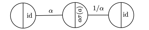
As an illustrative example, consider a neuron $n$ with the Swish activation function and weighted sum of inputs $a$, $n$'s spective weighted sums of inputs $a_{1}, a_{2}, a_{3}$, see the figure below:

Another aspect that is worth to stress is that for all the above mentioned trainable activation functions a gradient descent method based on backpropagation was used to train all the parameters of the networks; however, to train the activation function parameters the standard backpropagation formulas have to be suitable and specifically adapted to each trainable activation function.

2. Functions based on Ensemble Methods

With the expression "ensemble methods" we refer to any technique merging together different functions. Basically, each of these techniques uses:

• A set of basis functions, which can contain fixed-shape functions or trainable functions or both;

• A combination model, which defines how the basis functions are combined together.

2.1 Linear Combination of One-to-one Functions

In a nutshell, this kind of trainable activation function can be reduced to

$$f(a) = \sum_{i=1}^{h} \alpha_{i}\cdot g_{i}(a)$$

where $g_{1}, g_{2}, ..., g_{h}$ are one-to-one mapping functions, that is $g_{i}: \mathbb{R} \rightarrow \mathbb{R}, \forall 1 \leq i \leq h$ and $\alpha_{i}$ are weights associated with the functions, usually learned by data.

All the works reviewed in this section can be reduced to this general form. However, we distinguish at least two different ways in which they are presented originally:

• The linear combination of functions can be expressed as a neural network.
• The trainable activation functions are expressed using an analytical form.

Adaptive Activation Functions

Qian et al. propose different mixtures of the ELU and ReLU functions able to obtain a final activation function learned from data:

• Mixed activation: $\Phi_{M}(a) = p \cdot LReLU(a) + (1-p) \cdot ELU(a)$ with $p \in [0, 1]$ learned from data.
• Gated activation: $\Phi_{G}(a) = \sigma(\beta a) \cdot LReLU(a) + (1-\sigma(\beta a)) \cdot ELU(a)$ with $\sigma(\cdot)$ the sigmoid function and $\beta$ learned from data.
• Hierarchical activation: this function is composed of a three-level subnetwork, where each input unit $u$ is connected to $n$ units, and every pair of nodes are combined similarly as in gated activation. At the same time, the last layer takes the maximum of the middle-level unit. So, the hierarchical organization can be formalized as follows:

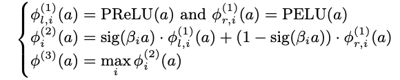
where $\phi_{l, i}^{(1)}(a)$ is for the units of the first level, with $i = 1, 2, \cdots , m$, $\phi_{i}^{(2)}(a)$ is used for the $i$-th unit of the second level, and $\phi^{(3)}(a)$ is for the third level; the final activation function is $\Phi_{H}(a) = \phi_{l}^{(3)}(a)$.

Variable Activation Function

Apicella et al. propose a class of trainable activation functions which are expressed in terms of sub-networks with only one hidden layer, relying on the consideration that a one-hidden layer neural network can approximate arbitrarily well any continuous functional mapping from one finite-dimensional space to another, enabling the resulting function to assume "any" shape.

In a netshell, their activation function is modeled as a non-linear activation function $f$ with a neuron with an identity activation function which sends its output to a one-hidden-layer sub-network with just one output neuron having, in turn, an identity as an output function. It can be expressed as:

$$VAF(a) = \sum_{j=1}^{k} \beta_{j} g(\alpha_{j} a + \alpha_{0j}) + \beta_{0}$$

where $g$ is a fixed-shape activation function, $k$ is a hyper-parameter that determines the number of hidden nodes of the subnetwork and $\alpha_{j}, \alpha_{0j}, \beta_{j}, \beta_{0}$ are parameters learned from the data during the training process.

Kernel-based Activation Function

This activation function is proposed by Scardapane et al., it is modeled in terms of a kernel expansion:

$$KAF(a) = \sum_{i=1}^D \alpha_{i} k(a, d_{i})$$

where $\alpha_{1}, \alpha_{2}, \ldots ,\alpha_{D}$ are the trainable parameters, $k$ is a kernel function $k: \R \times \R \rightarrow \R$ and $d_{1}, d_{2}, \ldots ,d_{D}$ are the dictionary elements, sampled from the real line for simpleness.

Adaptive Blending Unit

This work is proposed by Sutfeld et al., it combines together a set of different functions in a linear way as follows:

$$ABU(a) = \sum_{i=1}^{k} \alpha_{i} \cdot f_{i}(a)$$

with $(\alpha_{1}, \alpha_{2}, \ldots, \alpha_{k})$ parameters to learn and $(f_{1}(\cdot), f_{2}(\cdot), \ldots, f_{k}(\cdot))$ a set of activation functions that is, in the original study, composed of Tanh, ELU, ReLU, Id, and Swish. The $\alpha$ parameters are all initialized with $\frac{1}{k}$ and are constrained using four different normalization schemes.

Adaptive Piecewise Linear Units

Agostinelli et al. propose a class of activation functions, which can be modeled as a sum of hinge-shaped functions that results in a different piecewise linear activation function for every neuron:

$$ APL(a) = max(0, a) + \sum_{i=1}^{k} w_{k} max(0, -a + b_{k})$$

where $k$ is a hyper-parameter and $w_{k}, b_{k}$ are parameters learned during the network training.

It should be point out that the total overhead in terms of number of parameters to learn compared with a classic NN with $n$ units is $2 \cdot k \cdot n$, so the number of parameters increases with the number of hidden units and, for a large input, the learned function trends to behave as a ReLU function, reducing the expressiveness of the learned activation functions.

Harmon & Klabjan Activation Ensembles

Some studies try to define activation functions using different available activation functions rather than creating an entirely new function. Klabjan and Harmon provide a method to allow the network to choose the best activation function from a predefined set $F = {f^{(1), f^{(2), \ldots ,f^{(k)}}$, or some combination of those.

The activation function proposed by them works on single mini-batch, i.e. its input is tuple $\bf{a}^{(u)} = (a_{1}^{(u)}, a_{2}^{(u)}, \ldots, a_{B}^{(u)})$ where every $a_{i}^{(u)}, 1 \leq i \leq B$ refers to the unit $u$ on the $i$-th element of the mini-batch. The proposed activationn function is based on a sum of normalized functions weighted by a set of learned weights; the resulting activation function $\Phi(a)$ of $\bf{a}^{(u)}$ has the form:

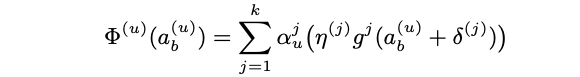
where $\alpha_{u}^{j}$ is a weight value for the $u$-th unit and the $j$-th function, $\eta^{(j)}$ and $\delta^{(j)}$ are inserted to allow the network choosing to leave the activation in its original state if the performance is particularly good and

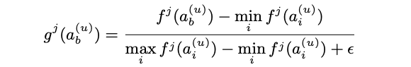
where $\epsilon$ is a small number.

The authors emphasize that, during the experiments, many neurons favored the ReLU function since the respective $a_{i}^{(u)}$ had greater magnitude compared with the others. The learning of the $\alpha$ values was done in terms of an optimization problem with the the additional approach, which seems to require additional computational costs due to the resolution of a new optimization problem together with the standard network learning procedure.

S-Shaped ReLU

Taking inspiration from the Webner-Fechner law and Stevens law, Jin et al. designed an activation S-shape function determined by three linear functions:

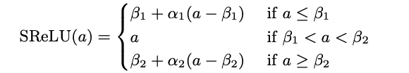
where $b_{1}, w_{1}, b_{2}, w_{2}$ are parameters that can be learned together with the other network parameters. SReLU can learn both convex and non-convex functions, differently from other trainable approaches like Maxout unit that can learn just convex function. Furthermore, this function can approximate also ReLU when $b_{2} \geq 0, w_{2} = 1, b_{1} = 0, w_{1} = 0$ or LReLU/PReLU when $b_{2} \geq 0, w_{2} = 1, b_{1} = 0, w_{1} > 0$.

Discussion

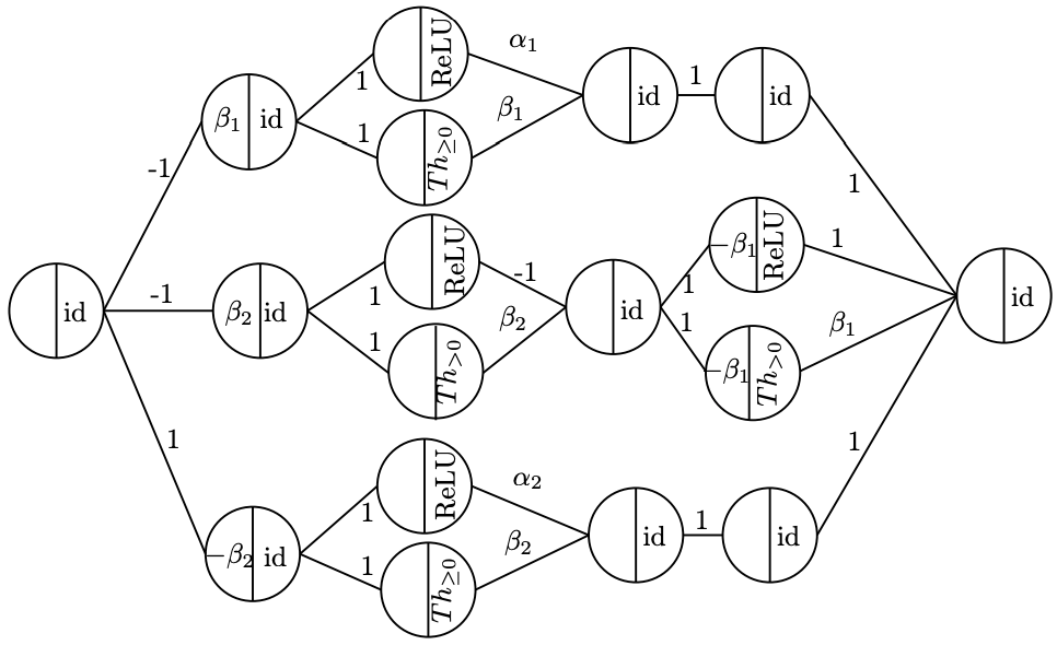
As mentioned above, a linear combination of one-to-one functions is always expressible as a linear combination of one-to-one mappings. Due to this common property, several of them can be expressed in terms of feed-forward neural networks (FFNN). For these functions that a natural equivalent formulationn in terms of subnetworks exists, making these architectures not only easy to integrate into the main models, but also easier to study using the general rules of feed-forward neural networks.

For instance, the SReLU can be expressed as:

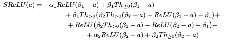
where $Th_{>0}(x) = 1 - Th_{\geq 0}(-x)$ and $\beta_{1} \geq \beta_{2}$. So the SReLU functions can be expressed as FFNN with constraints on the parameters and the inner activation function as illustrated in the figure below.

Summary

In this blog, we give a brief introduction to the trainable activation functions. We have divided the proposed functions into two main categories:paremeterized standard functions and functions based on ensemble methods. The latter has been refined further by isolating another activation function family: linear combination of one-to-one functions.

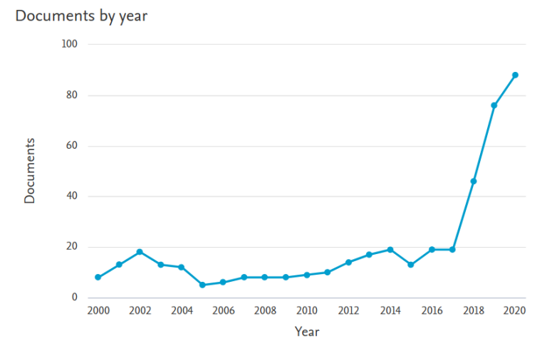
In literature we usually find the expression "trainable activation functions", however the expressions "learnable", "adaptive" or "adaptable" activationn functions are also used interchangeably. In recent years there has been a particular interest in this topic, the general trend can be seen from the figure below.

So far, we have completed three blogs in a row to give a brief introduction to the commonly used activation functions. Hope these are helpful to you, happy machine learning!